5. Uncertainties

Import Python libraries Hide code cell content

from __future__ import annotations

import itertools
import json
import logging
import os
import tarfile
from collections import defaultdict
from textwrap import wrap

import jax.numpy as jnp
import matplotlib.pyplot as plt
import numpy as np
import plotly.graph_objects as go
import sympy as sp
import yaml
from ampform.kinematics.phasespace import is_within_phasespace
from ampform.sympy import PoolSum
from IPython.display import Latex, Markdown
from matplotlib import cm
from matplotlib.ticker import FuncFormatter, MultipleLocator
from plotly.subplots import make_subplots
from scipy.interpolate import griddata
from tensorwaves.function.sympy import create_function
from tensorwaves.interface import DataSample, ParametrizedFunction
from tqdm.auto import tqdm

from polarimetry import formulate_polarimetry
from polarimetry.amplitude import AmplitudeModel
from polarimetry.data import (
    create_data_transformer,
    generate_meshgrid_sample,
    generate_phasespace_sample,
)
from polarimetry.function import integrate_intensity, sub_intensity
from polarimetry.io import (
    export_polarimetry_field,
    mute_jax_warnings,
    perform_cached_doit,
    perform_cached_lambdify,
)
from polarimetry.lhcb import (
    ParameterBootstrap,
    load_model_builder,
    load_model_parameters,
)
from polarimetry.lhcb.particle import load_particles
from polarimetry.plot import add_watermark, use_mpl_latex_fonts

logging.getLogger("polarimetry.io").setLevel(logging.INFO)
mute_jax_warnings()
FUNCTION_CACHE: dict[sp.Expr, ParametrizedFunction] = {}
UNFOLDED_POOLSUM_CACHE: dict[PoolSum, sp.Expr] = {}

NO_TQDM = "EXECUTE_NB" in os.environ
if NO_TQDM:
    logging.getLogger().setLevel(logging.ERROR)
    logging.getLogger("polarimetry.io").setLevel(logging.ERROR)

5.1. Model loading

Formulate models Hide code cell source

model_file = "../data/model-definitions.yaml"
particles = load_particles("../data/particle-definitions.yaml")
reference_subsystem = 1
with open(model_file) as f:
    model_titles = list(yaml.safe_load(f))

models = {}
for title in tqdm(model_titles, desc="Formulating models", disable=NO_TQDM):
    amplitude_builder = load_model_builder(model_file, particles, model_id=title)
    model = amplitude_builder.formulate(reference_subsystem)
    imported_parameter_values = load_model_parameters(
        model_file, model.decay, title, particles
    )
    model.parameter_defaults.update(imported_parameter_values)
    models[title] = model

Unfold symbolic expressions Hide code cell source

def unfold_poolsum(expr: PoolSum) -> sp.Expr:
    unfolded_expr = UNFOLDED_POOLSUM_CACHE.get(expr)
    if unfolded_expr is None:
        unfolded_expr = expr.doit()
        UNFOLDED_POOLSUM_CACHE[expr] = unfolded_expr
        return unfolded_expr
    return unfolded_expr


nominal_model_title = "Default amplitude model"
nominal_model = models[nominal_model_title]
unfolded_exprs = {}
for title, model in tqdm(
    models.items(), desc="Unfolding expressions", disable=NO_TQDM
):
    amplitude_builder = load_model_builder(model_file, particles, model_id=title)
    polarimetry_exprs = formulate_polarimetry(amplitude_builder, reference_subsystem)
    folded_exprs = {f"alpha_{i}": expr for i, expr in zip("xyz", polarimetry_exprs)}
    folded_exprs["intensity"] = model.intensity
    unfolded_exprs[title] = {
        key: perform_cached_doit(unfold_poolsum(expr).xreplace(model.amplitudes))
        for key, expr in tqdm(
            folded_exprs.items(), disable=NO_TQDM, leave=False, postfix=title
        )
    }

Identify unique expressions Hide code cell source

expression_hashes = {
    title: hash(exprs["intensity"]) for title, exprs in unfolded_exprs.items()
}
table = R"""
$$
\begin{array}{rllr}
  && \textbf{Model description} & n\textbf{ ops.} \\
  \hline
"""
for i, (title, expressions) in enumerate(unfolded_exprs.items()):
    expr = expressions["intensity"]
    h = hash(expr)
    for j, v in enumerate(expression_hashes.values()):
        if h == v:
            break
    same_as = ""
    if i != j:
        same_as = f"= {j}"
    ops = sp.count_ops(expr)
    title = "".join(Rf"\text{{{t}}}\\ " for t in wrap(title, width=56))
    title = Rf"\begin{{array}}{{l}}{title}\end{{array}}"
    title = title.replace("^", R"\^{}")
    table += Rf"  \mathbf{{{i}}} & {same_as} & {title} & {ops:,} \\ \hline" "\n"
table += R"""\end{array}
$$
"""

n_models = len(models)
n_unique_hashes = len(set(expression_hashes.values()))
src = Rf"""
Of the {n_models} models, there are {n_unique_hashes} with a unique expression tree.
"""
if NO_TQDM:
    src += "\n:::{dropdown} Show number of mathematical operations per model\n"
src += table
if NO_TQDM:
    src += "\n:::"
Markdown(src.strip())

Of the 18 models, there are 9 with a unique expression tree.

Show number of mathematical operations per model

\[\begin{split} \begin{array}{rllr} && \textbf{Model description} & n\textbf{ ops.} \\ \hline \mathbf{0} & & \begin{array}{l}\text{Default amplitude model}\\ \end{array} & 43,198 \\ \hline \mathbf{1} & = 0 & \begin{array}{l}\text{Alternative amplitude model with K(892) with free mass}\\ \text{and width}\\ \end{array} & 43,198 \\ \hline \mathbf{2} & = 0 & \begin{array}{l}\text{Alternative amplitude model with L(1670) with free mass}\\ \text{and width}\\ \end{array} & 43,198 \\ \hline \mathbf{3} & = 0 & \begin{array}{l}\text{Alternative amplitude model with L(1690) with free mass}\\ \text{and width}\\ \end{array} & 43,198 \\ \hline \mathbf{4} & = 0 & \begin{array}{l}\text{Alternative amplitude model with D(1232) with free mass}\\ \text{and width}\\ \end{array} & 43,198 \\ \hline \mathbf{5} & = 0 & \begin{array}{l}\text{Alternative amplitude model with L(1600), D(1600),}\\ \text{D(1700) with free mass and width}\\ \end{array} & 43,198 \\ \hline \mathbf{6} & = 0 & \begin{array}{l}\text{Alternative amplitude model with free L(1405) Flatt'e}\\ \text{widths, indicated as G1 (pK channel) and G2 (Sigmapi)}\\ \end{array} & 43,198 \\ \hline \mathbf{7} & & \begin{array}{l}\text{Alternative amplitude model with L(1800) contribution}\\ \text{added with free mass and width}\\ \end{array} & 44,222 \\ \hline \mathbf{8} & & \begin{array}{l}\text{Alternative amplitude model with L(1810) contribution}\\ \text{added with free mass and width}\\ \end{array} & 46,782 \\ \hline \mathbf{9} & & \begin{array}{l}\text{Alternative amplitude model with D(1620) contribution}\\ \text{added with free mass and width}\\ \end{array} & 44,222 \\ \hline \mathbf{10} & & \begin{array}{l}\text{Alternative amplitude model in which a Relativistic}\\ \text{Breit-Wigner is used for the K(700) contribution}\\ \end{array} & 43,470 \\ \hline \mathbf{11} & = 0 & \begin{array}{l}\text{Alternative amplitude model with K(700) with free mass}\\ \text{and width}\\ \end{array} & 43,198 \\ \hline \mathbf{12} & & \begin{array}{l}\text{Alternative amplitude model with K(1410) contribution}\\ \text{added with mass and width from PDG2020}\\ \end{array} & 46,780 \\ \hline \mathbf{13} & & \begin{array}{l}\text{Alternative amplitude model in which a Relativistic}\\ \text{Breit-Wigner is used for the K(1430) contribution}\\ \end{array} & 43,470 \\ \hline \mathbf{14} & = 0 & \begin{array}{l}\text{Alternative amplitude model with K(1430) with free width}\\ \end{array} & 43,198 \\ \hline \mathbf{15} & & \begin{array}{l}\text{Alternative amplitude model with an additional overall}\\ \text{exponential form factor exp(-alpha q\^{}2) multiplying Bugg}\\ \text{lineshapes. The exponential parameter is indicated as}\\ \text{``alpha''}\\ \end{array} & 43,582 \\ \hline \mathbf{16} & = 0 & \begin{array}{l}\text{Alternative amplitude model with free radial parameter d}\\ \text{for the Lc resonance, indicated as dLc}\\ \end{array} & 43,198 \\ \hline \mathbf{17} & & \begin{array}{l}\text{Alternative amplitude model obtained using LS couplings}\\ \end{array} & 110,839 \\ \hline \end{array} \end{split}\]

Convert to numerical functions Hide code cell source

def cached_lambdify(expr: sp.Expr, model: AmplitudeModel) -> ParametrizedFunction:
    func = FUNCTION_CACHE.get(expr)
    if func is None:
        func = perform_cached_lambdify(
            expr,
            parameters=model.parameter_defaults,
            backend="jax",
        )
        FUNCTION_CACHE[expr] = func
    str_parameters = {str(k): v for k, v in model.parameter_defaults.items()}
    func.update_parameters(str_parameters)
    return func


jax_functions = {}
original_parameters: dict[str, dict[str, complex | float | int]] = {}
progress_bar = tqdm(desc="Lambdifying to JAX", disable=NO_TQDM, total=len(models))
for title, model in models.items():
    progress_bar.set_postfix_str(title)
    jax_functions[title] = {
        key: cached_lambdify(expr, model)
        for key, expr in unfolded_exprs[title].items()
    }
    original_parameters[title] = dict(jax_functions[title]["intensity"].parameters)
    progress_bar.update()
progress_bar.set_postfix_str("")
progress_bar.close()

5.2. Statistical uncertainties

5.2.1. Parameter bootstrapping

n_bootstraps = 100
nominal_functions = jax_functions[nominal_model_title]
bootstrap = ParameterBootstrap(model_file, nominal_model.decay, nominal_model_title)
bootstrap_parameters = bootstrap.create_distribution(n_bootstraps, seed=0)

n_events = 100_000
transformer = create_data_transformer(nominal_model)
phsp_sample = generate_phasespace_sample(nominal_model.decay, n_events, seed=0)
phsp_sample = transformer(phsp_sample)

Compute polarimeter field and intensities (statistics & systematics) Hide code cell source

resonances = [chain.resonance for chain in nominal_model.decay.chains]
nominal_parameters = dict(original_parameters[nominal_model_title])
stat_grids = defaultdict(list)
stat_decay_rates = defaultdict(list)
for i in tqdm(
    range(n_bootstraps),
    desc="Computing polarimetry and intensities for parameter combinations",
    disable=NO_TQDM,
):
    new_parameters = {k: v[i] for k, v in bootstrap_parameters.items()}
    for key, func in nominal_functions.items():
        func.update_parameters(nominal_parameters)
        func.update_parameters(new_parameters)
        stat_grids[key].append(func(phsp_sample).real)
    I_tot = integrate_intensity(stat_grids["intensity"][-1])
    for resonance in resonances:
        res_filter = resonance.name.replace("(", R"\(").replace(")", R"\)")
        I_sub = sub_intensity(
            nominal_functions["intensity"], phsp_sample, [res_filter]
        )
        stat_decay_rates[resonance.name].append(I_sub / I_tot)

stat_intensities = jnp.array(stat_grids["intensity"])
stat_polarimetry = jnp.array([stat_grids[f"alpha_{i}"] for i in "xyz"])
stat_polarimetry_norm = jnp.sqrt(jnp.sum(stat_polarimetry**2, axis=0))
stat_decay_rates = {k: jnp.array(v) for k, v in stat_decay_rates.items()}

5.2.2. Mean and standard deviations

assert stat_intensities.shape == (n_bootstraps, n_events)
assert stat_polarimetry.shape == (3, n_bootstraps, n_events)
assert stat_polarimetry_norm.shape == (n_bootstraps, n_events)
n_bootstraps, n_events

(100, 100000)

Compute statistical measures (mean, std, etc.) Hide code cell source

stat_alpha_mean = [
    jnp.mean(stat_polarimetry_norm, axis=0),
    *jnp.mean(stat_polarimetry, axis=1),
]
stat_alpha_std = [
    jnp.std(stat_polarimetry_norm, axis=0),
    *jnp.std(stat_polarimetry, axis=1),
]

stat_alpha_times_I_mean = [
    jnp.mean(stat_polarimetry_norm * stat_intensities, axis=0),
    *jnp.mean(stat_polarimetry * stat_intensities, axis=1),
]
stat_alpha_times_I_std = [
    jnp.std(stat_polarimetry_norm * stat_intensities, axis=0),
    *jnp.std(stat_polarimetry * stat_intensities, axis=1),
]
stat_alpha_times_I_mean = jnp.array(stat_alpha_times_I_mean)
stat_alpha_times_I_std = jnp.array(stat_alpha_times_I_std)

stat_intensity_mean = jnp.mean(stat_intensities, axis=0)
stat_intensity_std = jnp.std(stat_intensities, axis=0)

5.2.3. Distributions

Define grid for plotting Hide code cell source

def interpolate_to_grid(values: np.ndarray, method: str = "linear"):
    return griddata(POINTS, values, (X, Y))


resolution = 200
POINTS = np.transpose(
    [
        phsp_sample["sigma1"],
        phsp_sample["sigma2"],
    ]
)
grid_sample = generate_meshgrid_sample(nominal_model.decay, resolution)
X = np.array(grid_sample["sigma1"])
Y = np.array(grid_sample["sigma2"])

Code for indicating Dalitz region Hide code cell content

def create_contour(phsp: DataSample) -> jnp.ndarray:
    # See also https://compwa-org.rtfd.io/report/017.html
    m0, m1, m2, m3, s1, s2 = sp.symbols("m(:4) sigma(1:3)", nonnegative=True)
    filter_expr = is_within_phasespace(
        s1,
        s2,
        nominal_model.parameter_defaults[m0],
        nominal_model.parameter_defaults[m1],
        nominal_model.parameter_defaults[m2],
        nominal_model.parameter_defaults[m3],
        outside_value=0,
    ).doit()
    filter_func = create_function(filter_expr, backend="jax")
    return filter_func(contour_sample)  # noqa: F821


def draw_dalitz_contour(
    ax, color: str = "black", width: float = 0.1, **kwargs
) -> None:
    ax.contour(
        X_CONTOUR,
        Y_CONTOUR,
        Z_CONTOUR,
        colors=color,
        linewidths=width,
        **kwargs,
    )


contour_sample = generate_meshgrid_sample(nominal_model.decay, resolution=500)
X_CONTOUR = np.array(contour_sample["sigma1"])
Y_CONTOUR = np.array(contour_sample["sigma2"])
Z_CONTOUR = create_contour(contour_sample)
del contour_sample, create_contour

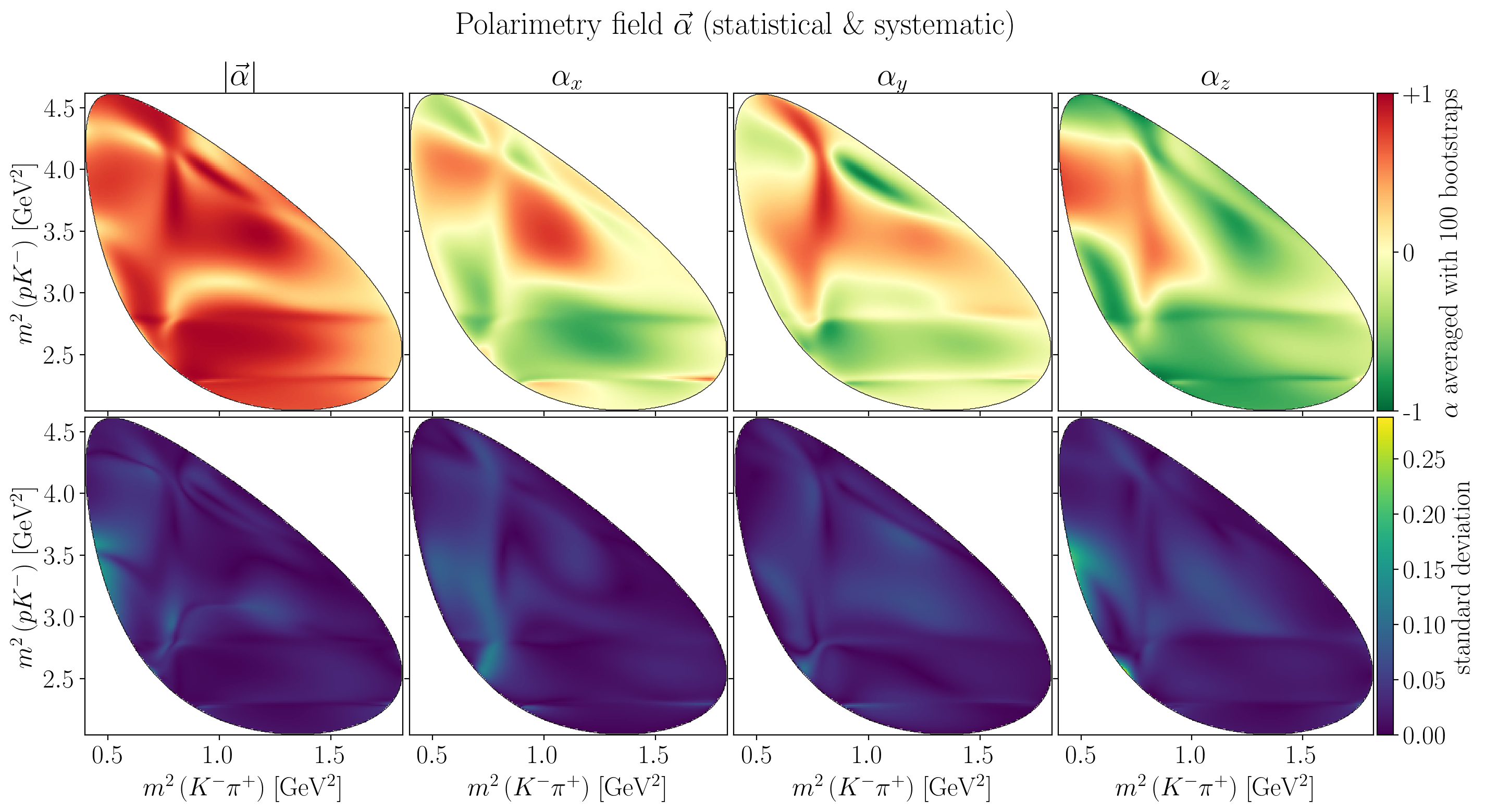
Show code cell source Hide code cell source

%config InlineBackend.figure_formats = ['png']
plt.rcdefaults()
use_mpl_latex_fonts()
plt.rc("font", size=18)
fig, axes = plt.subplots(
    dpi=200,
    figsize=(16.7, 8),
    gridspec_kw={"width_ratios": [1, 1, 1, 1.18]},
    ncols=4,
    nrows=2,
    sharex=True,
    sharey=True,
)
plt.subplots_adjust(hspace=0.02, wspace=0.02)
fig.suptitle(R"Polarimetry field $\vec\alpha$ (statistical \& systematic)")
s1_label = R"$m^2\left(K^-\pi^+\right)$ [GeV$^2$]"
s2_label = R"$m^2\left(pK^-\right)$ [GeV$^2$]"
s3_label = R"$m^2\left(p\pi^+\right)$ [GeV$^2$]"
axes[0, 0].set_ylabel(s2_label)
axes[1, 0].set_ylabel(s2_label)

global_max_std = max(map(jnp.nanmax, stat_alpha_std))
for i in range(4):
    if i != 0:
        title = Rf"$\alpha_{'xyz'[i-1]}$"
    else:
        title = R"$\left|\vec\alpha\right|$"
    axes[0, i].set_title(title)

    draw_dalitz_contour(axes[0, i], zorder=10)
    Z = interpolate_to_grid(stat_alpha_mean[i])
    mesh = axes[0, i].pcolormesh(X, Y, Z, cmap=cm.RdYlGn_r)
    mesh.set_clim(vmin=-1, vmax=+1)
    if axes[0, i] is axes[0, -1]:
        c_bar = fig.colorbar(mesh, ax=axes[0, i], pad=0.01)
        c_bar.ax.set_ylabel(Rf"$\alpha$ averaged with {n_bootstraps} bootstraps")
        c_bar.ax.set_yticks([-1, 0, +1])
        c_bar.ax.set_yticklabels(["-1", "0", "+1"])

    draw_dalitz_contour(axes[1, i], zorder=10)
    Z = interpolate_to_grid(stat_alpha_std[i])
    mesh = axes[1, i].pcolormesh(X, Y, Z)
    mesh.set_clim(vmin=0, vmax=global_max_std)
    axes[1, i].set_xlabel(s1_label)
    if axes[1, i] is axes[1, -1]:
        c_bar = fig.colorbar(mesh, ax=axes[1, i], pad=0.01)
        c_bar.ax.set_ylabel("standard deviation")
plt.show()

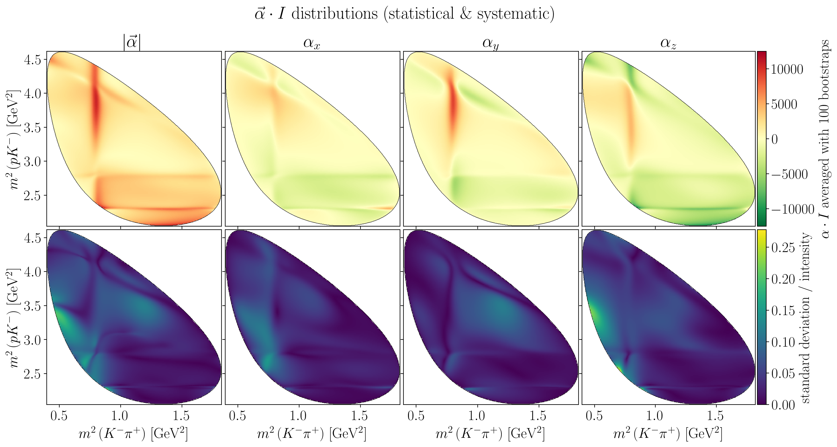
Show code cell source Hide code cell source

%config InlineBackend.figure_formats = ['png']
fig, axes = plt.subplots(
    dpi=200,
    figsize=(16.7, 8),
    gridspec_kw={"width_ratios": [1, 1, 1, 1.18]},
    ncols=4,
    nrows=2,
    sharex=True,
    sharey=True,
)
plt.subplots_adjust(hspace=0.02, wspace=0.02)
fig.suptitle(R"$\vec\alpha \cdot I$ distributions (statistical \& systematic)")
axes[0, 0].set_ylabel(s2_label)
axes[1, 0].set_ylabel(s2_label)

global_max_mean = jnp.nanmax(jnp.abs(stat_alpha_times_I_mean))
global_max_std = jnp.nanmax(stat_alpha_times_I_std / stat_intensity_mean)
for i in range(4):
    if i != 0:
        title = Rf"$\alpha_{'xyz'[i-1]}$"
    else:
        title = R"$\left|\vec\alpha\right|$"
    axes[0, i].set_title(title)
    axes[1, i].set_xlabel(s1_label)

    draw_dalitz_contour(axes[0, i], zorder=10)
    Z = interpolate_to_grid(stat_alpha_times_I_mean[i])
    mesh = axes[0, i].pcolormesh(X, Y, Z, cmap=cm.RdYlGn_r)
    mesh.set_clim(vmin=-global_max_mean, vmax=+global_max_mean)
    if axes[0, i] is axes[0, -1]:
        c_bar = fig.colorbar(mesh, ax=axes[0, i], pad=0.01)
        c_bar.ax.set_ylabel(
            Rf"$\alpha \cdot I$ averaged with {n_bootstraps} bootstraps"
        )

    draw_dalitz_contour(axes[1, i], zorder=10)
    Z = interpolate_to_grid(stat_alpha_times_I_std[i] / stat_intensity_mean)
    mesh = axes[1, i].pcolormesh(X, Y, Z)
    mesh.set_clim(vmin=0, vmax=global_max_std)
    if axes[1, i] is axes[1, -1]:
        c_bar = fig.colorbar(mesh, ax=axes[1, i], pad=0.01)
        c_bar.ax.set_ylabel("standard deviation / intensity")
plt.show()

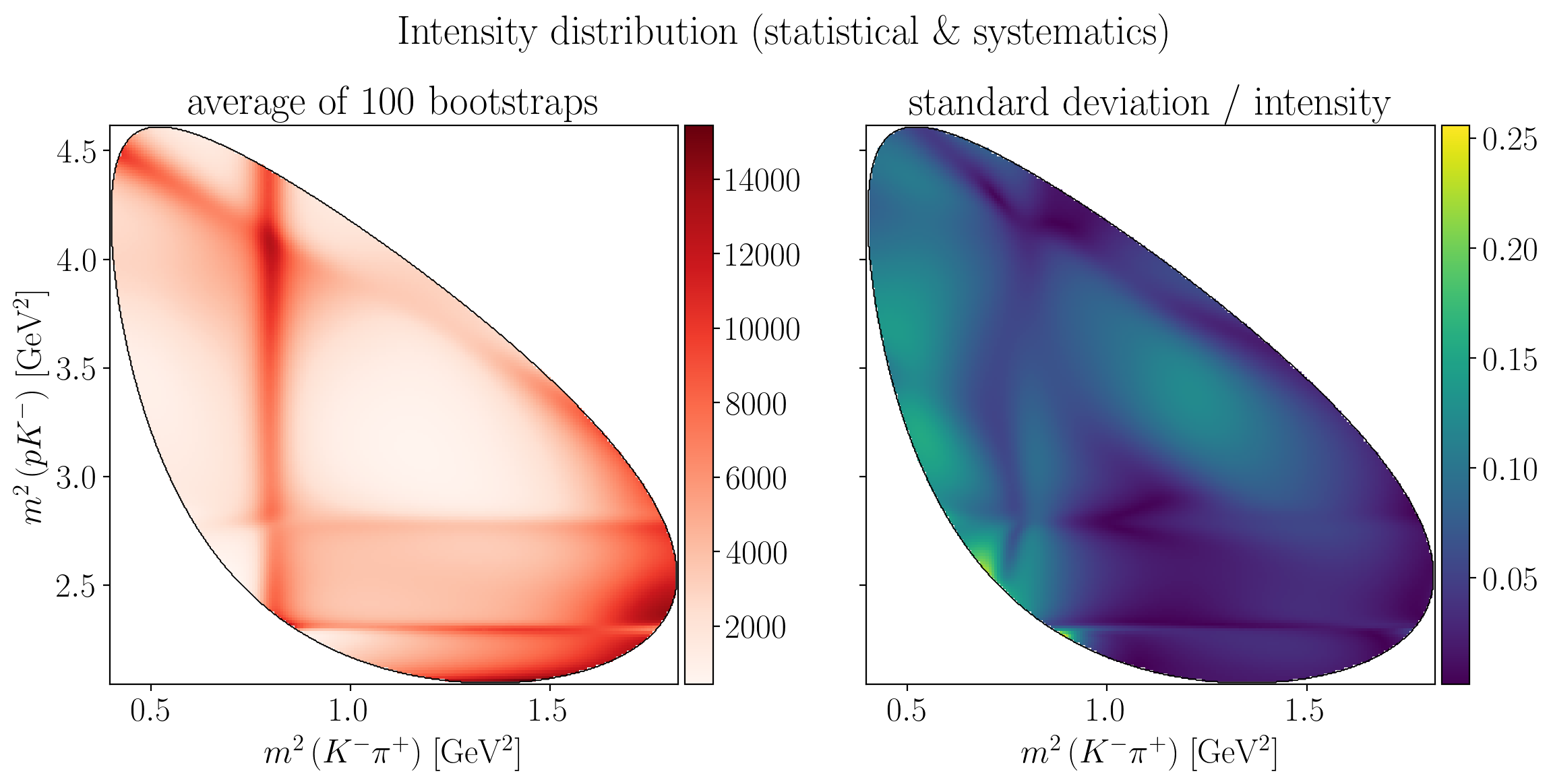
Show code cell source Hide code cell source

%config InlineBackend.figure_formats = ['png']
fig, (ax1, ax2) = plt.subplots(
    dpi=200,
    figsize=(12, 6.2),
    ncols=2,
    sharey=True,
)
fig.suptitle(R"Intensity distribution (statistical \& systematics)", y=0.95)
ax1.set_xlabel(s1_label)
ax2.set_xlabel(s1_label)
ax1.set_ylabel(s2_label)

Z = interpolate_to_grid(stat_intensity_mean)
mesh = ax1.pcolormesh(X, Y, Z, cmap=cm.Reds)
fig.colorbar(mesh, ax=ax1, pad=0.01)
draw_dalitz_contour(ax1, width=0.2)
ax1.set_title(f"average of {n_bootstraps} bootstraps")

Z = interpolate_to_grid(stat_intensity_std / stat_intensity_mean)
mesh = ax2.pcolormesh(X, Y, Z)
fig.colorbar(mesh, ax=ax2, pad=0.01)
draw_dalitz_contour(ax2, width=0.2)
ax2.set_title("standard deviation / intensity")
fig.tight_layout()
plt.show()

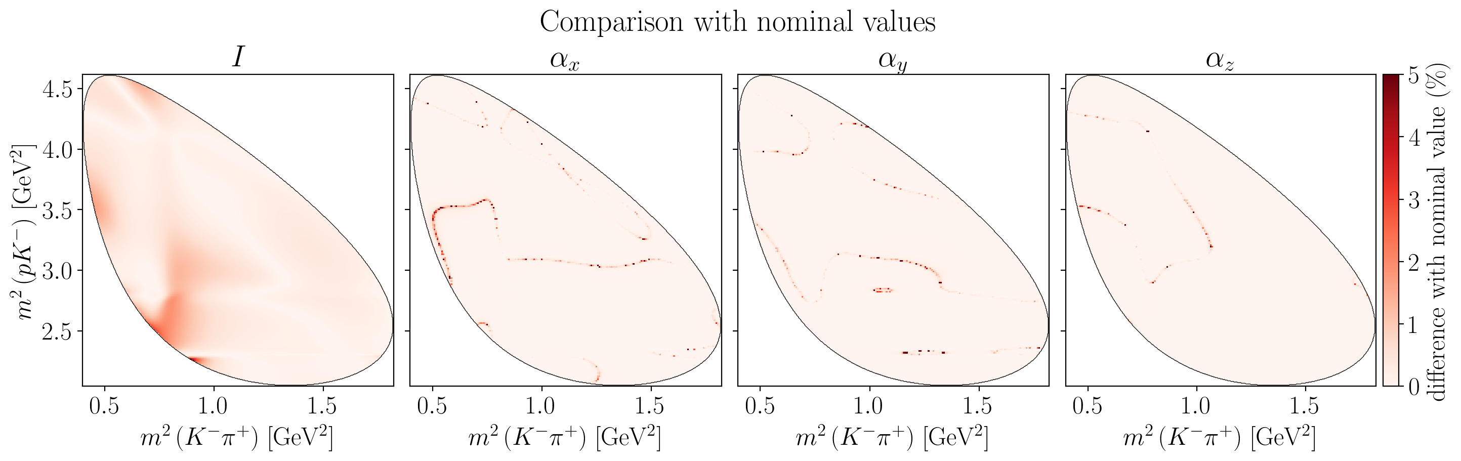
5.2.4. Comparison with nominal values

Compute nominal values Hide code cell source

for func in nominal_functions.values():
    func.update_parameters(nominal_parameters)
nominal_intensity = nominal_functions["intensity"](phsp_sample)
nominal_polarimetry = jnp.array(
    [nominal_functions[f"alpha_{i}"](phsp_sample).real for i in "xyz"]
)
nominal_polarimetry_norm = jnp.sqrt(jnp.sum(nominal_polarimetry**2, axis=0))

Show code cell source Hide code cell source

%config InlineBackend.figure_formats = ['png']
fig, axes = plt.subplots(
    dpi=200,
    figsize=(17.3, 4),
    gridspec_kw={"width_ratios": [1, 1, 1, 1.2]},
    ncols=4,
    sharey=True,
)
plt.subplots_adjust(hspace=0.2, wspace=0.05)
fig.suptitle("Comparison with nominal values", y=1.04)
axes[0].set_ylabel(s2_label)
for ax in axes:
    ax.set_xlabel(s1_label)

vmax = 5.0  # %
for i in range(4):
    if i != 0:
        title = Rf"$\alpha_{'xyz'[i-1]}$"
        z_values = jnp.abs(
            (stat_alpha_mean[i] - nominal_polarimetry[i - 1])
            / nominal_polarimetry[i - 1]
        )
    else:
        title = "$I$"
        z_values = 100 * jnp.abs(
            (stat_intensity_mean - nominal_intensity) / nominal_intensity
        )
    axes[i].set_title(title)

    draw_dalitz_contour(axes[i], zorder=10)
    Z = interpolate_to_grid(z_values)
    mesh = axes[i].pcolormesh(X, Y, Z, cmap=cm.Reds)
    mesh.set_clim(vmin=0, vmax=vmax)
    if axes[i] is axes[-1]:
        c_bar = fig.colorbar(mesh, ax=axes[i], pad=0.02)
        c_bar.ax.set_ylabel(R"difference with nominal value (\%)")

plt.show()

5.3. Systematic uncertainties

Show code cell content Hide code cell content

syst_grids = defaultdict(list)
syst_decay_rates = defaultdict(list)
progress_bar = tqdm(desc="Computing systematics", disable=NO_TQDM, total=len(models))
for title, model in models.items():
    progress_bar.set_postfix_str(title)
    for key, func in jax_functions[title].items():
        func.update_parameters(original_parameters[title])
        syst_grids[key].append(func(phsp_sample).real)
    I_tot = integrate_intensity(syst_grids["intensity"][-1])
    intensity_func = jax_functions[title]["intensity"]
    for resonance in resonances:
        res_filter = resonance.name.replace("(", R"\(").replace(")", R"\)")
        I_sub = sub_intensity(intensity_func, phsp_sample, [res_filter])
        syst_decay_rates[resonance.name].append(I_sub / I_tot)
    progress_bar.update()
progress_bar.set_postfix_str("")
progress_bar.close()

syst_intensities = jnp.array(syst_grids["intensity"])
syst_polarimetry = jnp.array([syst_grids[f"alpha_{i}"] for i in "xyz"])
syst_polarimetry_norm = jnp.sqrt(jnp.sum(syst_polarimetry**2, axis=0))
syst_decay_rates = {k: jnp.array(v) for k, v in syst_decay_rates.items()}

5.3.1. Mean and standard deviations

n_models = len(models)
assert syst_intensities.shape == (n_models, n_events)
assert syst_polarimetry.shape == (3, n_models, n_events)
assert syst_polarimetry_norm.shape == (n_models, n_events)
n_models, n_events

(18, 100000)

Compute statistical measures (mean, std, etc.) Hide code cell source

syst_alpha_mean = [
    jnp.mean(syst_polarimetry_norm, axis=0),
    *jnp.mean(syst_polarimetry, axis=1),
]
alpha_diff_with_model_0 = [
    syst_polarimetry_norm - syst_polarimetry_norm[0],
    *(syst_polarimetry - syst_polarimetry[:, None, 0]),
]

syst_alpha_mean = jnp.array(syst_alpha_mean)
alpha_diff_with_model_0 = jnp.array(alpha_diff_with_model_0)

assert alpha_diff_with_model_0.shape == (4, n_models, n_events)
assert jnp.nanmax(alpha_diff_with_model_0[:, 0]) == 0.0
alpha_syst_extrema = jnp.abs(alpha_diff_with_model_0).max(axis=1)

syst_polarimetry_times_I = [
    syst_polarimetry_norm * syst_intensities,
    *(syst_polarimetry * syst_intensities),
]
syst_polarimetry_times_I = jnp.array(syst_polarimetry_times_I)


syst_alpha_times_I_mean = syst_polarimetry_times_I.mean(axis=1)
syst_alpha_times_I_diff = (
    syst_polarimetry_times_I - syst_polarimetry_times_I[:, None, 0]
)
assert syst_alpha_times_I_diff.shape == (4, n_models, n_events)
assert jnp.nanmax(syst_alpha_times_I_diff[:, 0]) == 0.0
syst_alpha_times_I_extrema = jnp.abs(syst_alpha_times_I_diff).max(axis=1)

intensity_diff_with_model_0 = syst_intensities - syst_intensities[0]
intensity_extrema = jnp.nanmax(intensity_diff_with_model_0, axis=0)

5.3.2. Distributions

Show 1D projections of each model Hide code cell content

def plot_intensity_distributions(sigma: int) -> None:
    original_font_size = plt.rcParams["font.size"]
    use_mpl_latex_fonts()
    plt.rc("font", size=10)
    n_subplots = n_models - 1
    nrows = int(np.floor(np.sqrt(n_subplots)))
    ncols = int(np.ceil(n_subplots / nrows))
    fig, axes = plt.subplots(
        figsize=2.0 * np.array([ncols, nrows]),
        dpi=200,
        ncols=ncols,
        nrows=nrows,
        sharex=True,
        sharey=True,
    )
    fig.subplots_adjust(hspace=0, wspace=0, bottom=0.1, left=0.06)
    x_label = {1: s1_label, 2: s2_label, 3: s3_label}[sigma]
    fig.text(0.5, 0.04, x_label, ha="center")
    fig.text(0.04, 0.5, "$I$ (normalized)", va="center", rotation="vertical")
    for ax in axes.flatten()[n_subplots:]:
        fig.delaxes(ax)
    n_bins = 80
    nominal_bin_values, bin_edges = jnp.histogram(
        phsp_sample[f"sigma{sigma}"],
        weights=syst_intensities[0],
        bins=n_bins,
        density=True,
    )
    for i, (ax, intensities) in enumerate(
        zip(axes.flatten(), syst_intensities[1:]), 1
    ):
        ax.set_title(f"Model {i}", y=0.01)
        ax.set_yticks([])
        bin_values, _ = jnp.histogram(
            phsp_sample[f"sigma{sigma}"],
            weights=intensities,
            bins=n_bins,
            density=True,
        )
        ax.fill_between(
            bin_edges[:-1],
            bin_values,
            alpha=0.5,
            step="pre",
        )
        ax.step(
            x=bin_edges[:-1],
            y=nominal_bin_values,
            linewidth=0.3,
            color="red",
        )
    fig.savefig(f"_images/intensity-distributions-sigma{sigma}.svg")
    plt.show()
    use_mpl_latex_fonts()
    plt.rc("font", size=original_font_size)


%config InlineBackend.figure_formats = ['svg']
plot_intensity_distributions(1)
plot_intensity_distributions(2)
plot_intensity_distributions(3)

Show code cell source Hide code cell source

%config InlineBackend.figure_formats = ['png']
fig, axes = plt.subplots(
    dpi=200,
    figsize=(16.7, 8),
    gridspec_kw={"width_ratios": [1, 1, 1, 1.18]},
    ncols=4,
    nrows=2,
    sharex=True,
    sharey=True,
)
plt.subplots_adjust(hspace=0.02, wspace=0.02)
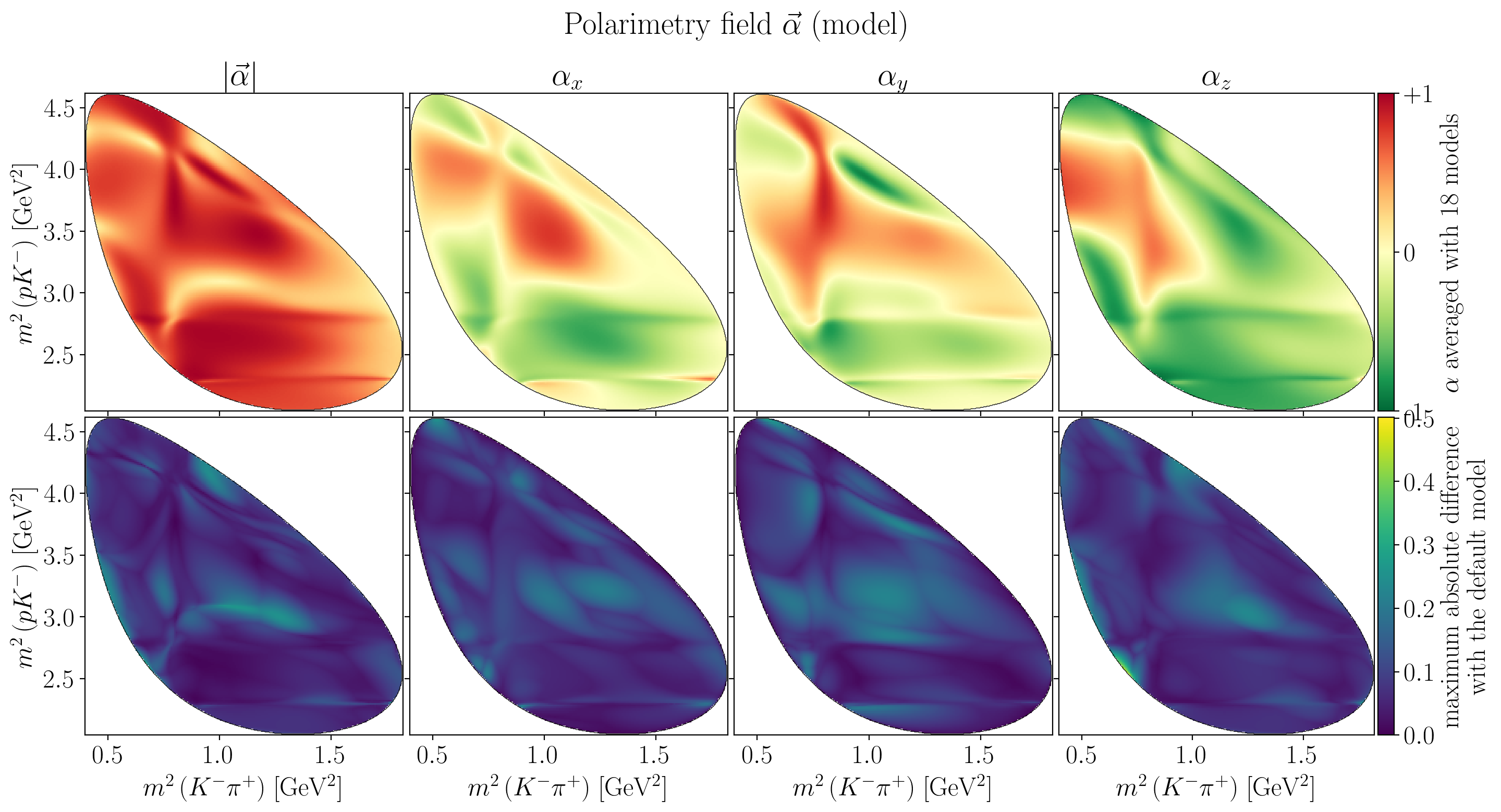
fig.suptitle(R"Polarimetry field $\vec\alpha$ (model)")
axes[0, 0].set_ylabel(s2_label)
axes[1, 0].set_ylabel(s2_label)

global_max_std = jnp.nanmax(alpha_syst_extrema)
for i in range(4):
    if i != 0:
        title = Rf"$\alpha_{'xyz'[i-1]}$"
    else:
        title = R"$\left|\vec\alpha\right|$"
    axes[0, i].set_title(title)

    draw_dalitz_contour(axes[0, i], zorder=10)
    Z = interpolate_to_grid(syst_alpha_mean[i])
    mesh = axes[0, i].pcolormesh(X, Y, Z, cmap=cm.RdYlGn_r)
    mesh.set_clim(vmin=-1, vmax=+1)
    if axes[0, i] is axes[0, -1]:
        c_bar = fig.colorbar(mesh, ax=axes[0, i], pad=0.01)
        c_bar.ax.set_ylabel(Rf"$\alpha$ averaged with {n_models} models")
        c_bar.ax.set_yticks([-1, 0, +1])
        c_bar.ax.set_yticklabels(["-1", "0", "+1"])

    draw_dalitz_contour(axes[1, i], zorder=10)
    Z = interpolate_to_grid(alpha_syst_extrema[i])
    mesh = axes[1, i].pcolormesh(X, Y, Z)
    mesh.set_clim(vmin=0, vmax=global_max_std)
    axes[1, i].set_xlabel(s1_label)
    if axes[1, i] is axes[1, -1]:
        c_bar = fig.colorbar(mesh, ax=axes[1, i], pad=0.01)
        c_bar.ax.set_ylabel("maximum absolute difference\nwith the default model")
plt.show()

Show code cell source Hide code cell source

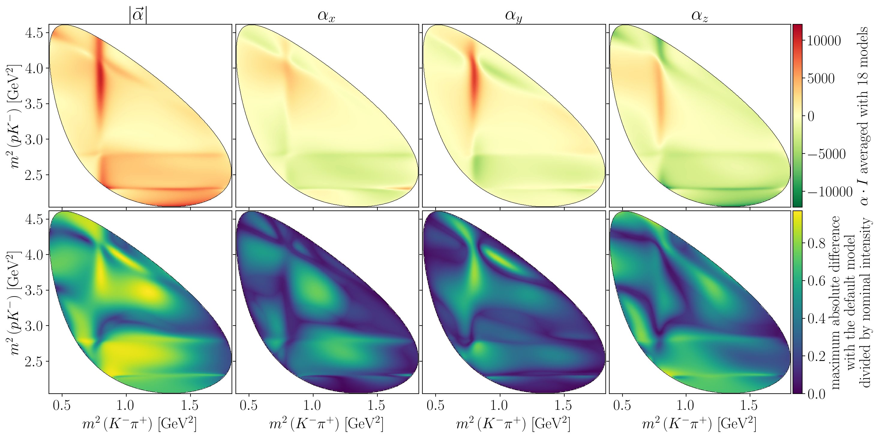
%config InlineBackend.figure_formats = ['png']
fig, axes = plt.subplots(
    dpi=200,
    figsize=(16.7, 8),
    gridspec_kw={"width_ratios": [1, 1, 1, 1.18]},
    ncols=4,
    nrows=2,
    sharex=True,
    sharey=True,
)
plt.subplots_adjust(hspace=0.02, wspace=0.02)
axes[0, 0].set_ylabel(s2_label)
axes[1, 0].set_ylabel(s2_label)

syst_intensity_mean = jnp.mean(syst_intensities, axis=0)
global_max_mean = jnp.nanmax(jnp.abs(syst_alpha_times_I_mean))
global_max_diff = jnp.nanmax(syst_alpha_times_I_extrema / syst_intensity_mean)
for i in range(4):
    if i != 0:
        title = Rf"$\alpha_{'xyz'[i-1]}$"
    else:
        title = R"$\left|\vec\alpha\right|$"
    axes[0, i].set_title(title)
    axes[1, i].set_xlabel(s1_label)

    draw_dalitz_contour(axes[0, i], zorder=10)
    Z = interpolate_to_grid(syst_alpha_times_I_mean[i])
    mesh = axes[0, i].pcolormesh(X, Y, Z, cmap=cm.RdYlGn_r)
    mesh.set_clim(vmin=-global_max_mean, vmax=+global_max_mean)
    if axes[0, i] is axes[0, -1]:
        c_bar = fig.colorbar(mesh, ax=axes[0, i], pad=0.01)
        c_bar.ax.set_ylabel(Rf"$\alpha \cdot I$ averaged with {n_models} models")

    draw_dalitz_contour(axes[1, i], zorder=10)
    Z = interpolate_to_grid(syst_alpha_times_I_extrema[i] / syst_intensity_mean)
    mesh = axes[1, i].pcolormesh(X, Y, Z)
    mesh.set_clim(vmin=0, vmax=global_max_diff)
    if axes[1, i] is axes[1, -1]:
        c_bar = fig.colorbar(mesh, ax=axes[1, i], pad=0.01)
        c_bar.ax.set_ylabel(
            "maximum absolute difference\n"
            "with the default model\n"
            "divided by nominal intensity"
        )
plt.show()

Show code cell source Hide code cell source

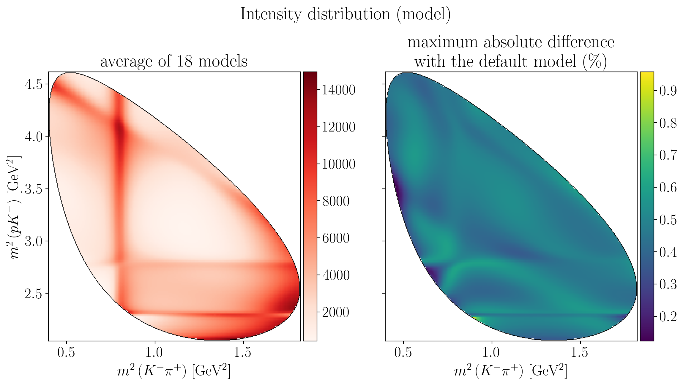
%config InlineBackend.figure_formats = ['png']
fig, (ax1, ax2) = plt.subplots(
    dpi=200,
    figsize=(12, 6.9),
    ncols=2,
    sharey=True,
)
fig.suptitle("Intensity distribution (model)", y=0.95)
ax1.set_xlabel(s1_label)
ax2.set_xlabel(s1_label)
ax1.set_ylabel(s2_label)

Z = interpolate_to_grid(syst_intensity_mean)
mesh = ax1.pcolormesh(X, Y, Z, cmap=cm.Reds)
fig.colorbar(mesh, ax=ax1, pad=0.01)
draw_dalitz_contour(ax1, width=0.2)
ax1.set_title(f"average of {n_models} models")

Z = interpolate_to_grid(intensity_extrema / syst_intensity_mean)
mesh = ax2.pcolormesh(X, Y, Z)
fig.colorbar(mesh, ax=ax2, pad=0.01)
draw_dalitz_contour(ax2, width=0.2)
ax2.set_title("maximum absolute difference\n" R"with the default model (\%)")
fig.tight_layout()
plt.show()

5.4. Uncertainty on polarimetry

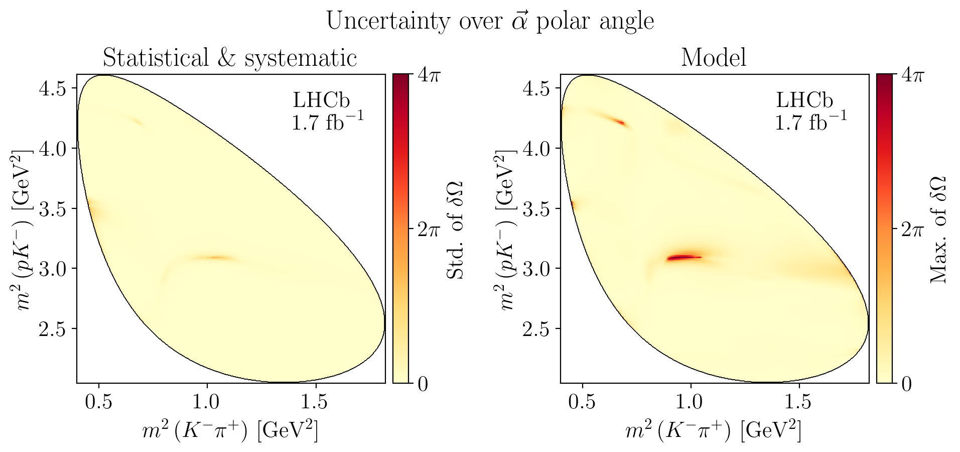
For each bootstrap or alternative model \(i\), we compute the angle between each aligned polarimeter vector \(\vec\alpha_i\) and the one from the nominal model, \(\vec\alpha_0\):

\[ \cos\theta_i = \frac{\vec \alpha_i \cdot \vec \alpha_0}{|\alpha_i||\alpha_0|}. \]

The solid angle can then be computed as:

\[ \delta\Omega = \int_0^{2\pi}\int_0^{\theta} \mathrm{d}\phi \, \mathrm{d}\cos\theta = 2\pi\left(1-\cos\theta\right). \]

The statistical uncertainty is given by taking the standard deviation on the \(\delta\Omega\) distribution and the systematic uncertainty is given by taking finding \(\theta_\mathrm{max} = \max\theta_i\) and computing \(\delta\Omega_\mathrm{max}\) from that.

Show code cell source Hide code cell source

def dot(array1: jnp.ndarray, array2: jnp.ndarray, axis=0) -> jnp.ndarray:
    return jnp.sum(array1 * array2, axis=axis)


def norm(array: jnp.ndarray, axis=0) -> jnp.ndarray:
    return jnp.sqrt(dot(array, array, axis=axis))


def compute_theta(polarimetry: jnp.ndarray) -> jnp.ndarray:
    return jnp.arccos(
        dot(polarimetry, nominal_polarimetry[:, None])
        / (norm(polarimetry) * norm(nominal_polarimetry))
    )


def compute_solid_angle(theta: jnp.ndarray) -> jnp.ndarray:
    return 2 * jnp.pi * (1 - jnp.cos(theta))


stat_theta = compute_theta(stat_polarimetry)
syst_theta = compute_theta(syst_polarimetry)
assert stat_theta.shape == (n_bootstraps, n_events)
assert syst_theta.shape == (n_models, n_events)

stat_solid_angle = jnp.nanstd(compute_solid_angle(stat_theta), axis=0)
syst_solid_angle = jnp.nanmax(compute_solid_angle(syst_theta), axis=0)


def plot_angle_uncertainties(watermark: bool, titles: bool) -> None:
    plt.ioff()
    fig, axes = plt.subplots(
        dpi=200,
        figsize=(11, 4),
        ncols=2,
    )
    fig.subplots_adjust(wspace=0.3)
    ax1, ax2 = axes
    if titles:
        fig.suptitle(R"Uncertainty over $\vec\alpha$ polar angle", y=1.04)
        ax1.set_title(R"Statistical \& systematic")
        ax2.set_title("Model")
    for ax in axes:
        ax.set_box_aspect(1)
        ax.set_xlabel(s1_label)
        ax.set_ylabel(s2_label)
        draw_dalitz_contour(ax, width=0.2, zorder=10)

    Z = interpolate_to_grid(stat_solid_angle)
    mesh = ax1.pcolormesh(X, Y, Z, cmap=plt.cm.YlOrRd)
    mesh.set_clim(0, 4 * np.pi)
    c_bar = fig.colorbar(mesh, ax=ax1, pad=0.02)
    c_bar.ax.set_ylabel(R"Std. of $\delta\Omega$")
    c_bar.ax.set_yticks([0, 2 * np.pi, 4 * np.pi])
    c_bar.ax.set_yticklabels(["$0$", R"$2\pi$", R"$4\pi$"])

    Z = interpolate_to_grid(syst_solid_angle)
    mesh = ax2.pcolormesh(X, Y, Z, cmap=plt.cm.YlOrRd)
    mesh.set_clim(0, 4 * np.pi)
    c_bar = fig.colorbar(mesh, ax=ax2, pad=0.02)
    c_bar.ax.set_ylabel(R"Max. of $\delta\Omega$")
    c_bar.ax.set_yticks([0, 2 * np.pi, 4 * np.pi])
    c_bar.ax.set_yticklabels(["$0$", R"$2\pi$", R"$4\pi$"])
    output_file = "polarimetry-field-angle-uncertainties"
    if watermark:
        output_file += "-watermark"
        add_watermark_to_uncertainties(ax1)
        add_watermark_to_uncertainties(ax2)
    if titles:
        output_file += "-with-titles"
    fig.savefig(f"_static/images/{output_file}.png", bbox_inches="tight")
    if watermark and titles:
        plt.show()
    plt.close(fig)
    plt.ion()


def add_watermark_to_uncertainties(ax) -> None:
    add_watermark(ax, 0.70, 0.82, fontsize=16)


%config InlineBackend.figure_formats = ['png']
plt.rcdefaults()
use_mpl_latex_fonts()
plt.rc("font", size=16)

boolean_combinations = list(itertools.product(*2 * [[False, True]]))
for watermark, titles in tqdm(boolean_combinations, disable=NO_TQDM):
    plot_angle_uncertainties(watermark, titles)

Show code cell source Hide code cell source

stat_alpha_difference = norm(stat_polarimetry - nominal_polarimetry[:, None])
syst_alpha_difference = norm(syst_polarimetry - nominal_polarimetry[:, None])
nominal_polarimetry_norm = norm(nominal_polarimetry[:, None])
stat_alpha_rel_difference = 100 * stat_alpha_difference / nominal_polarimetry_norm
syst_alpha_rel_difference = 100 * syst_alpha_difference / nominal_polarimetry_norm
assert stat_alpha_rel_difference.shape == (n_bootstraps, n_events)
assert syst_alpha_rel_difference.shape == (n_models, n_events)


def create_figure(titles: bool):
    fig, axes = plt.subplots(
        dpi=200,
        figsize=(11.5, 4),
        ncols=2,
    )
    fig.subplots_adjust(wspace=0.4)
    ax1, ax2 = axes
    if titles:
        fig.suptitle(R"Uncertainty over $\left|\vec\alpha\right|$", y=1.04)
        ax1.set_title(R"Statistical \& systematic")
        ax2.set_title("Model")
    for ax in axes:
        ax.set_box_aspect(1)
        ax.set_xlabel(s1_label)
        ax.set_ylabel(s2_label)
        draw_dalitz_contour(ax, width=0.2)
    return fig, (ax1, ax2)


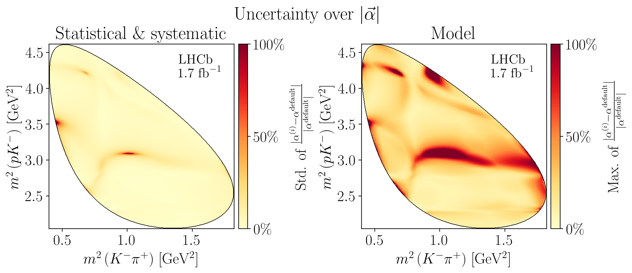
def plot_norm_rel_uncertainties(watermark: bool, titles: bool) -> None:
    plt.ioff()
    fig, (ax1, ax2) = create_figure(titles)
    Z = interpolate_to_grid(jnp.nanstd(stat_alpha_rel_difference, axis=0))
    mesh = ax1.pcolormesh(X, Y, Z, cmap=plt.cm.YlOrRd)
    mesh.set_clim(0, 100)
    c_bar = fig.colorbar(mesh, ax=ax1, pad=0.02)
    c_bar.ax.set_ylabel(
        R"Std. of"
        R" $\frac{|\alpha^{(i)}-\alpha^\mathrm{default}|}{|\alpha^\mathrm{default}|}$"
    )
    c_bar.ax.set_yticks([0, 50, 100])
    c_bar.ax.set_yticklabels([R"0\%", R"50\%", R"100\%"])
    Z = interpolate_to_grid(jnp.nanmax(syst_alpha_rel_difference, axis=0))
    mesh = ax2.pcolormesh(X, Y, Z, cmap=plt.cm.YlOrRd)
    mesh.set_clim(0, 100)
    c_bar = fig.colorbar(mesh, ax=ax2, pad=0.02)
    c_bar.ax.set_ylabel(
        R"Max. of"
        R" $\frac{|\alpha^{(i)}-\alpha^\mathrm{default}|}{|\alpha^\mathrm{default}|}$"
    )
    c_bar.ax.set_yticks([0, 50, 100])
    c_bar.ax.set_yticklabels([R"0\%", R"50\%", R"100\%"])
    output_file = "polarimetry-field-norm-uncertainties-relative"
    if watermark:
        output_file += "-watermark"
        add_watermark_to_uncertainties(ax1)
        add_watermark_to_uncertainties(ax2)
    if titles:
        output_file += "-with-titles"
    fig.savefig(f"_static/images/{output_file}.png", bbox_inches="tight")
    if watermark and titles:
        plt.show()
    plt.close(fig)
    plt.ion()


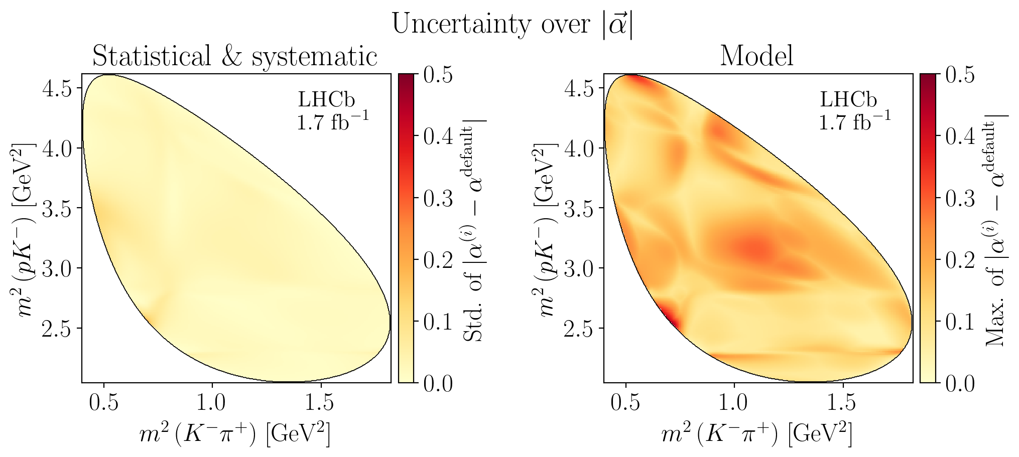
def plot_norm_uncertainties(watermark: bool, titles: bool) -> None:
    plt.ioff()
    vmax = 0.5
    fig, (ax1, ax2) = create_figure(titles)
    Z = interpolate_to_grid(jnp.nanstd(stat_alpha_difference, axis=0))
    mesh = ax1.pcolormesh(X, Y, Z, cmap=plt.cm.YlOrRd)
    c_bar = fig.colorbar(mesh, ax=ax1, pad=0.02)
    mesh.set_clim(0, vmax)
    c_bar.ax.set_ylabel(R"Std. of $|\alpha^{(i)}-\alpha^\mathrm{default}|$")
    Z = interpolate_to_grid(jnp.nanmax(syst_alpha_difference, axis=0))
    mesh = ax2.pcolormesh(X, Y, Z, cmap=plt.cm.YlOrRd)
    mesh.set_clim(0, vmax)
    c_bar = fig.colorbar(mesh, ax=ax2, pad=0.02)
    c_bar.ax.set_ylabel(R"Max. of $|\alpha^{(i)}-\alpha^\mathrm{default}|$")
    output_file = "polarimetry-field-norm-uncertainties"
    if watermark:
        output_file += "-watermark"
        add_watermark_to_uncertainties(ax1)
        add_watermark_to_uncertainties(ax2)
    if titles:
        output_file += "-with-titles"
    fig.savefig(f"_static/images/{output_file}.png", bbox_inches="tight")
    if watermark and titles:
        plt.show()
    plt.close(fig)
    plt.ion()


%config InlineBackend.figure_formats = ['png']
plt.rcdefaults()
use_mpl_latex_fonts()
plt.rc("font", size=18)

for watermark, titles in tqdm(boolean_combinations, disable=NO_TQDM):
    plot_norm_rel_uncertainties(watermark, titles)
    plot_norm_uncertainties(watermark, titles)

5.5. Decay rates

Show code cell source Hide code cell source

with open("../data/observable-references.yaml") as f:
    data = yaml.load(f, Loader=yaml.SafeLoader)
lhcb_values = {
    k: tuple(float(v) for v in row.split(" ± "))
    for k, row in data[nominal_model_title]["rate"].items()
}

src = R"""
\begin{array}{l|c|c}
\textbf{Resonance} & \textbf{Decay rate} & \textbf{LHCb} \\
\hline
"""
for resonance in resonances:
    ff_statistical = 100 * stat_decay_rates[resonance.name]
    ff_systematics = 100 * syst_decay_rates[resonance.name]
    ff_nominal = f"{ff_systematics[0]:.2f}"
    ff_stat = f"{ff_statistical.std():.2f}"
    ff_syst_min = f"{(ff_systematics[1:]-ff_systematics[0]).min():+.2f}"
    ff_syst_max = f"{(ff_systematics[1:]-ff_systematics[0]).max():+.2f}"
    src += f"{resonance.latex} & "
    src += Rf"{ff_nominal} \pm {ff_stat}_{{{ff_syst_min}}}^{{{ff_syst_max}}} & "
    lhcb_value, lhcb_stat, lhcb_syst, _ = lhcb_values[resonance.name]
    src += Rf"{lhcb_value} \pm {lhcb_stat} \pm {lhcb_syst} \\" "\n"
src += R"\end{array}"
Latex(src)

\[\begin{split}\begin{array}{l|c|c} \textbf{Resonance} & \textbf{Decay rate} & \textbf{LHCb} \\ \hline \Lambda(1405) & 7.78 \pm 0.43_{-2.53}^{+3.01} & 7.7 \pm 0.2 \pm 3.0 \\ \Lambda(1520) & 1.91 \pm 0.10_{-0.24}^{+0.04} & 1.86 \pm 0.09 \pm 0.23 \\ \Lambda(1600) & 5.16 \pm 0.28_{-1.93}^{+0.50} & 5.2 \pm 0.2 \pm 1.9 \\ \Lambda(1670) & 1.15 \pm 0.04_{-0.29}^{+0.06} & 1.18 \pm 0.06 \pm 0.32 \\ \Lambda(1690) & 1.16 \pm 0.01_{-0.33}^{+0.06} & 1.19 \pm 0.09 \pm 0.34 \\ \Lambda(2000) & 9.55 \pm 0.67_{-2.26}^{+0.83} & 9.58 \pm 0.27 \pm 0.93 \\ \Delta(1232) & 28.73 \pm 1.34_{-0.79}^{+1.76} & 28.6 \pm 0.29 \pm 0.76 \\ \Delta(1600) & 4.50 \pm 0.51_{-1.40}^{+0.93} & 4.5 \pm 0.3 \pm 1.5 \\ \Delta(1700) & 3.89 \pm 0.07_{-0.48}^{+0.94} & 3.9 \pm 0.2 \pm 0.94 \\ K(700) & 2.99 \pm 0.20_{-0.59}^{+0.91} & 3.02 \pm 0.16 \pm 0.92 \\ K(892) & 21.95 \pm 1.24_{-0.70}^{+0.59} & 22.14 \pm 0.23 \pm 0.64 \\ K(1430) & 14.70 \pm 0.80_{-2.67}^{+2.78} & 14.7 \pm 0.6 \pm 2.7 \\ \end{array}\end{split}\]

Show code cell source Hide code cell source

alignment = "c".join("" for _ in range(n_models) if i)
names = " & ".join(Rf"\textbf{{{i}}}" for i in range(n_models) if i)
src = Rf"""
$$
\begin{{array}}{{l|{alignment}}}
  \textbf{{Resonance}} & {names} \\
  \hline
"""
for resonance in resonances:
    ff_systematics = 100 * syst_decay_rates[resonance.name]
    src += f"  {resonance.latex:13s}"
    for ff_model in ff_systematics[1:]:
        diff = f"{ff_model-ff_systematics[0]:+.2f}"
        if ff_model == ff_systematics[1:].min():
            src += Rf" & \color{{blue}}{{{diff}}}"
        elif ff_model == ff_systematics[1:].max():
            src += Rf" & \color{{red}}{{{diff}}}"
        else:
            src += f" & {diff}"
    src += R" \\" "\n"
src += """\
\\end{array}
$$
"""
for i, title in enumerate(models):
    src += f"\n- **{i}**: {title}"
Markdown(src)

\[\begin{split} \begin{array}{l|ccccccccccccccccc} \textbf{Resonance} & \textbf{1} & \textbf{2} & \textbf{3} & \textbf{4} & \textbf{5} & \textbf{6} & \textbf{7} & \textbf{8} & \textbf{9} & \textbf{10} & \textbf{11} & \textbf{12} & \textbf{13} & \textbf{14} & \textbf{15} & \textbf{16} & \textbf{17} \\ \hline \Lambda(1405) & +0.11 & -0.14 & -0.01 & -0.33 & -0.99 & \color{red}{+3.01} & \color{blue}{-2.53} & -0.66 & -1.58 & -0.43 & -0.01 & -1.97 & -0.11 & -0.04 & -0.18 & +0.06 & -0.75 \\ \Lambda(1520) & +0.03 & +0.00 & +0.01 & +0.01 & \color{blue}{-0.24} & -0.01 & -0.04 & -0.08 & -0.06 & -0.06 & \color{red}{+0.04} & -0.15 & -0.00 & +0.00 & -0.09 & -0.00 & +0.03 \\ \Lambda(1600) & -0.02 & -0.09 & +0.13 & +0.22 & \color{red}{+0.50} & -0.09 & -0.30 & +0.23 & \color{blue}{-1.93} & -0.46 & +0.12 & -1.85 & -0.12 & -0.06 & +0.00 & -0.03 & +0.05 \\ \Lambda(1670) & -0.01 & \color{red}{+0.06} & +0.03 & +0.01 & -0.01 & -0.12 & \color{blue}{-0.29} & -0.03 & -0.11 & +0.05 & -0.01 & -0.03 & +0.01 & +0.00 & -0.03 & -0.01 & +0.02 \\ \Lambda(1690) & +0.00 & -0.00 & +0.04 & -0.13 & +0.01 & -0.06 & -0.04 & -0.26 & \color{blue}{-0.33} & -0.08 & -0.04 & \color{red}{+0.06} & +0.01 & +0.00 & -0.10 & -0.01 & -0.08 \\ \Lambda(2000) & +0.05 & +0.10 & -0.08 & -0.09 & +0.08 & -0.85 & \color{blue}{-2.26} & \color{red}{+0.83} & -0.93 & +0.31 & -0.23 & -0.86 & +0.35 & +0.19 & -1.40 & -0.02 & +0.30 \\ \Delta(1232) & -0.27 & +0.02 & +0.31 & \color{red}{+1.76} & -0.44 & -0.14 & +0.49 & -0.63 & -0.77 & +0.53 & -0.31 & +0.65 & +0.10 & +0.06 & \color{blue}{-0.79} & -0.25 & +0.24 \\ \Delta(1600) & +0.33 & -0.10 & -0.15 & -0.28 & +0.59 & -0.38 & \color{blue}{-1.40} & -0.29 & \color{red}{+0.93} & +0.03 & +0.05 & -0.58 & +0.07 & +0.04 & -0.10 & +0.01 & -0.26 \\ \Delta(1700) & -0.01 & +0.03 & -0.13 & +0.07 & +0.39 & \color{blue}{-0.48} & -0.15 & +0.82 & \color{red}{+0.94} & +0.18 & +0.05 & +0.75 & +0.03 & +0.01 & +0.23 & +0.01 & +0.10 \\ K(700) & +0.17 & -0.02 & +0.04 & +0.75 & +0.62 & \color{blue}{-0.59} & -0.31 & -0.06 & \color{red}{+0.91} & +0.56 & +0.25 & +0.42 & +0.10 & +0.07 & -0.06 & +0.01 & +0.26 \\ K(892) & -0.53 & -0.02 & -0.12 & -0.46 & -0.58 & +0.55 & \color{red}{+0.59} & -0.06 & +0.18 & +0.28 & -0.16 & +0.25 & -0.01 & +0.00 & -0.52 & +0.02 & \color{blue}{-0.70} \\ K(1430) & -0.29 & +0.07 & -0.50 & -0.03 & +0.18 & -0.76 & \color{red}{+2.78} & +2.40 & \color{blue}{-2.67} & +1.29 & +0.23 & -2.27 & +0.91 & +0.44 & +2.07 & -0.00 & +0.71 \\ \end{array} \end{split}\]

• 0: Default amplitude model

• 1: Alternative amplitude model with K(892) with free mass and width

• 2: Alternative amplitude model with L(1670) with free mass and width

• 3: Alternative amplitude model with L(1690) with free mass and width

• 4: Alternative amplitude model with D(1232) with free mass and width

• 5: Alternative amplitude model with L(1600), D(1600), D(1700) with free mass and width

• 6: Alternative amplitude model with free L(1405) Flatt’e widths, indicated as G1 (pK channel) and G2 (Sigmapi)

• 7: Alternative amplitude model with L(1800) contribution added with free mass and width

• 8: Alternative amplitude model with L(1810) contribution added with free mass and width

• 9: Alternative amplitude model with D(1620) contribution added with free mass and width

• 10: Alternative amplitude model in which a Relativistic Breit-Wigner is used for the K(700) contribution

• 11: Alternative amplitude model with K(700) with free mass and width

• 12: Alternative amplitude model with K(1410) contribution added with mass and width from PDG2020

• 13: Alternative amplitude model in which a Relativistic Breit-Wigner is used for the K(1430) contribution

• 14: Alternative amplitude model with K(1430) with free width

• 15: Alternative amplitude model with an additional overall exponential form factor exp(-alpha q^2) multiplying Bugg lineshapes. The exponential parameter is indicated as ``alpha’’

• 16: Alternative amplitude model with free radial parameter d for the Lc resonance, indicated as dLc

• 17: Alternative amplitude model obtained using LS couplings

5.6. Average polarimetry values

The components of the averaged polarimeter vector \(\overline{\alpha}\) are defined as:

\[ \overline{\alpha}_j = \int I_0\left(\tau\right) \alpha_j\left(\tau\right) \mathrm{d}^n \tau \; \big / \int I_0\left(\tau\right)\,\mathrm{d}^n \tau \]

The averages of the norm of \(\vec\alpha\) are computed as follows:

• \(\left|\overline{\alpha}\right| = \sqrt{\overline{\alpha_x}^2+\overline{\alpha_y}^2+\overline{\alpha_z}^2}\), with the statistical uncertainties added in quadrature and the systematic uncertainties by taking the same formula on the extrema values of each \(\overline{\alpha_j}\)

• \(\overline{\left|\alpha\right|} = \sqrt{\int I_0\left(\tau\right) \left|\vec\alpha\left(\tau\right)\right|^2 \mathrm{d}^n \tau \; \big / \int I_0\left(\tau\right)\,\mathrm{d}^n \tau}\)

Show code cell source Hide code cell source

def compute_weighted_average(v: jnp.ndarray, weights: jnp.ndarray) -> jnp.ndarray:
    return jnp.nansum(v * weights, axis=-1) / jnp.nansum(weights, axis=-1)


def compute_polar_coordinates(cartesian_vector: jnp.ndarray) -> jnp.ndarray:
    x, y, z = cartesian_vector
    norm = jnp.sqrt(jnp.sum(cartesian_vector**2, axis=0))
    theta = np.arccos(z / norm)
    phi = np.pi - np.arctan2(y, -x)
    return jnp.array([norm, theta, phi])


stat_weighted_alpha_norm = jnp.sqrt(
    compute_weighted_average(stat_polarimetry_norm**2, weights=stat_intensities)
)
stat_weighted_alpha = compute_weighted_average(
    stat_polarimetry,
    weights=stat_intensities,
)
stat_weighted_alpha_polar = compute_polar_coordinates(stat_weighted_alpha)
assert stat_weighted_alpha_norm.shape == (n_bootstraps,)
assert stat_weighted_alpha.shape == (3, n_bootstraps)
assert stat_weighted_alpha_polar.shape == (3, n_bootstraps)

syst_weighted_alpha_norm = jnp.sqrt(
    compute_weighted_average(syst_polarimetry_norm**2, weights=syst_intensities)
)
syst_weighted_alpha = compute_weighted_average(
    syst_polarimetry,
    weights=syst_intensities,
)
syst_weighted_alpha_polar = compute_polar_coordinates(syst_weighted_alpha)
assert syst_weighted_alpha_norm.shape == (n_models,)
assert syst_weighted_alpha.shape == (3, n_models)
assert syst_weighted_alpha_polar.shape == (3, n_models)

nominal_weighted_alpha_norm = syst_weighted_alpha_norm[0]
nominal_weighted_alpha = syst_weighted_alpha[:, 0]
nominal_weighted_alpha_polar = syst_weighted_alpha_polar[:, 0]

syst_weighted_alpha_norm_diff = (
    syst_weighted_alpha_norm - nominal_weighted_alpha_norm
)
syst_weighted_alpha_diff = (syst_weighted_alpha.T - nominal_weighted_alpha).T
syst_weighted_alpha_diff_polar = (
    syst_weighted_alpha_polar.T - nominal_weighted_alpha_polar
).T

stat_weighted_alpha_std = stat_weighted_alpha.std(axis=1)
syst_weighted_alpha_min = syst_weighted_alpha_diff.min(axis=1)
syst_weighted_alpha_max = syst_weighted_alpha_diff.max(axis=1)
stat_weighted_alpha_polar_std = stat_weighted_alpha_polar.std(axis=1)
syst_weighted_alpha_polar_min = syst_weighted_alpha_diff_polar.min(axis=1)
syst_weighted_alpha_polar_max = syst_weighted_alpha_diff_polar.max(axis=1)

Cartesian coordinates:

Show code cell source Hide code cell source

def render_cartesian_uncertainties(
    value, stat, syst_min, syst_max, plus: bool = True
) -> str:
    value *= 1e3
    stat *= 1e3
    syst_min *= 1e3
    syst_max *= 1e3
    if plus:
        val = f"{value:+.1f}"
    else:
        val = f"{value:.1f}"
    stat = f"{stat:.1f}"
    syst_min = f"-{abs(syst_min):.1f}"
    syst_max = f"+{abs(syst_max):.1f}"
    return (
        Rf"\left({val} \pm {stat}_{{{syst_min}}}^{{{syst_max}}} \right) \times"
        R" 10^{-3}"
    )


src = R"""
\begin{array}{ccr}
"""
for i in range(3):
    value = render_cartesian_uncertainties(
        nominal_weighted_alpha[i],
        stat_weighted_alpha_std[i],
        syst_weighted_alpha_min[i],
        syst_weighted_alpha_max[i],
    )
    src += Rf"  \overline{{\alpha_{'xyz'[i]}}} & = & {value} \\" "\n"

value = render_cartesian_uncertainties(
    nominal_weighted_alpha_norm,
    stat_weighted_alpha_norm.std(),
    syst_weighted_alpha_norm_diff.min(),
    syst_weighted_alpha_norm_diff.max(),
    plus=False,
)
src += Rf"  \overline{{\left|\alpha\right|}} & = & {value} \\"
src += R"\end{array}"
Latex(src)

\[\begin{split}\begin{array}{ccr} \overline{\alpha_x} & = & \left(-62.6 \pm 4.5_{-14.8}^{+8.4} \right) \times 10^{-3} \\ \overline{\alpha_y} & = & \left(+8.9 \pm 8.9_{-12.7}^{+9.1} \right) \times 10^{-3} \\ \overline{\alpha_z} & = & \left(-278.0 \pm 23.7_{-40.4}^{+12.6} \right) \times 10^{-3} \\ \overline{\left|\alpha\right|} & = & \left(669.4 \pm 9.3_{-10.4}^{+15.3} \right) \times 10^{-3} \\\end{array}\end{split}\]

Polar coordinates:

\[\begin{split} \begin{array}{lcl} \theta\left(\vec\alpha\right) &=& \arccos\left(\alpha_z \, \big/ \left|\alpha\right|\right) \\ \phi\left(\vec\alpha\right) &=& \pi - \mathrm{atan2}\left(\alpha_y, -\alpha_x\right) \end{array} \end{split}\]

Show code cell source Hide code cell source

def render_radian_angle_uncertainties(value, stat, syst_min, syst_max) -> str:
    val = f"{value:+.2f}"
    stat = f"{stat:.2f}"
    syst_min = f"-{abs(syst_min):.2f}"
    syst_max = f"+{abs(syst_max):.2f}"
    return Rf"{val} \pm {stat}_{{{syst_min}}}^{{{syst_max}}}\;\mathrm{{rad}}"


def render_angle_uncertainties(value, stat, syst_min, syst_max) -> str:
    value /= np.pi
    stat /= np.pi
    syst_min /= np.pi
    syst_max /= np.pi
    val = f"{value:+.3f}"
    stat = f"{stat:.3f}"
    syst_min = f"-{abs(syst_min):.3f}"
    syst_max = f"+{abs(syst_max):.3f}"
    return (
        Rf"\left({val} \pm {stat}_{{{syst_min}}}^{{{syst_max}}} \right) \times \pi"
    )


src = R"""
\begin{array}{ccl}
"""
labels = [
    R"\left|\overline{\alpha}\right|",
    R"\theta\left(\overline{\alpha}\right)",
    R"\phi\left(\overline{\alpha}\right)",
]
for i, label in enumerate(labels):
    renderer = (
        render_cartesian_uncertainties
        if i == 0
        else render_radian_angle_uncertainties
    )
    args = (
        nominal_weighted_alpha_polar[i],
        stat_weighted_alpha_polar_std[i],
        syst_weighted_alpha_polar_min[i],
        syst_weighted_alpha_polar_max[i],
    )
    src += Rf"  {label} & = & {renderer(*args)} \\" "\n"
    if i > 0:
        src += Rf"  & = & {render_angle_uncertainties(*args)} \\" "\n"

src += R"\end{array}"
Latex(src)

\[\begin{split}\begin{array}{ccl} \left|\overline{\alpha}\right| & = & \left(+285.1 \pm 24.0_{-13.8}^{+37.9} \right) \times 10^{-3} \\ \theta\left(\overline{\alpha}\right) & = & +2.92 \pm 0.01_{-0.04}^{+0.05}\;\mathrm{rad} \\ & = & \left(+0.929 \pm 0.002_{-0.011}^{+0.017} \right) \times \pi \\ \phi\left(\overline{\alpha}\right) & = & +3.00 \pm 0.14_{-0.09}^{+0.21}\;\mathrm{rad} \\ & = & \left(+0.955 \pm 0.045_{-0.028}^{+0.067} \right) \times \pi \\ \end{array}\end{split}\]

Averaged polarimeter values for each model (and the difference with the nominal model):

Show code cell source Hide code cell source

src = R"""
\begin{array}{r|rrrr|rrrr}
  \textbf{Model}
  & \overline{\alpha}_x & \overline{\alpha}_y & \overline{\alpha}_z & \overline{\left|\alpha\right|}
  & \Delta\overline{\alpha}_x & \Delta\overline{\alpha}_y & \Delta\overline{\alpha}_z
  & \Delta\overline{\left|\alpha\right|} \\
  \hline
"""
for i, title in enumerate(models):
    α = 1e3 * syst_weighted_alpha[:, i]
    abs_α = 1e3 * syst_weighted_alpha_norm[i]
    Δα = 1e3 * syst_weighted_alpha_diff[:, i]
    abs_Δα = 1e3 * syst_weighted_alpha_norm_diff[i]
    src += Rf"  \textbf{{{i}}}"
    src += Rf"  & {α[0]:+.1f} & {α[1]:+.1f} & {α[2]:+.1f} & {abs_α:.1f}"
    if i != 0:
        src += Rf"  & {Δα[0]:+.1f} & {Δα[1]:+.1f} & {Δα[2]:+.1f} & {abs_Δα:+.1f}"
    src += R"  \\" "\n"
    del i, title, α, abs_α, Δα, abs_Δα
src += R"\end{array}"
Latex(src)

\[\begin{split}\begin{array}{r|rrrr|rrrr} \textbf{Model} & \overline{\alpha}_x & \overline{\alpha}_y & \overline{\alpha}_z & \overline{\left|\alpha\right|} & \Delta\overline{\alpha}_x & \Delta\overline{\alpha}_y & \Delta\overline{\alpha}_z & \Delta\overline{\left|\alpha\right|} \\ \hline \textbf{0} & -62.6 & +8.9 & -278.0 & 669.4 \\ \textbf{1} & -61.6 & +8.5 & -279.4 & 670.7 & +1.0 & -0.4 & -1.4 & +1.3 \\ \textbf{2} & -62.9 & +9.1 & -278.4 & 669.8 & -0.3 & +0.2 & -0.5 & +0.4 \\ \textbf{3} & -58.4 & +7.4 & -276.2 & 667.7 & +4.2 & -1.5 & +1.8 & -1.6 \\ \textbf{4} & -69.3 & +9.5 & -277.2 & 666.9 & -6.6 & +0.6 & +0.8 & -2.5 \\ \textbf{5} & -70.7 & +9.6 & -277.4 & 668.7 & -8.0 & +0.8 & +0.6 & -0.6 \\ \textbf{6} & -69.7 & +9.1 & -281.7 & 673.0 & -7.1 & +0.2 & -3.8 & +3.7 \\ \textbf{7} & -77.4 & +18.0 & -305.4 & 671.4 & -14.8 & +9.1 & -27.5 & +2.1 \\ \textbf{8} & -55.8 & +10.9 & -284.6 & 675.5 & +6.8 & +2.0 & -6.7 & +6.1 \\ \textbf{9} & -66.9 & +4.4 & -290.4 & 672.8 & -4.3 & -4.5 & -12.4 & +3.5 \\ \textbf{10} & -56.4 & +2.4 & -265.4 & 659.0 & +6.2 & -6.5 & +12.6 & -10.4 \\ \textbf{11} & -64.7 & +9.3 & -278.6 & 670.4 & -2.1 & +0.4 & -0.6 & +1.0 \\ \textbf{12} & -75.1 & +1.8 & -283.4 & 663.5 & -12.5 & -7.1 & -5.4 & -5.8 \\ \textbf{13} & -61.8 & +8.1 & -277.3 & 668.8 & +0.9 & -0.8 & +0.7 & -0.6 \\ \textbf{14} & -62.2 & +8.7 & -277.6 & 669.2 & +0.5 & -0.2 & +0.4 & -0.2 \\ \textbf{15} & -54.2 & -3.8 & -318.4 & 684.6 & +8.4 & -12.7 & -40.4 & +15.3 \\ \textbf{16} & -62.1 & +8.2 & -278.1 & 669.5 & +0.5 & -0.7 & -0.1 & +0.2 \\ \textbf{17} & -58.1 & +12.1 & -278.6 & 666.5 & +4.5 & +3.2 & -0.6 & -2.9 \\ \end{array}\end{split}\]

Show code cell source Hide code cell source

src = R"""
\begin{array}{r|rrr|rrr}
  \textbf{Model}
  & 10^3 \cdot \left|\overline{\alpha}\right|
  & \theta\left(\overline{\alpha}\right) / \pi
  & \phi\left(\overline{\alpha}\right) / \pi
  & 10^3 \cdot \Delta\left|\overline{\alpha}\right|
  & \Delta\theta\left(\overline{\alpha}\right) / \pi
  & \Delta\phi\left(\overline{\alpha}\right) / \pi \\
  \hline
"""
for i, title in enumerate(models):
    α, θ, φ = syst_weighted_alpha_polar[:, i]
    Δα, Δθ, Δφ = syst_weighted_alpha_diff_polar[:, i]
    src += Rf"  \textbf{{{i}}}"
    src += Rf"  & {1e3*α:+.1f} & {θ/np.pi:+.3f} & {φ/np.pi:+.3f}"
    if i != 0:
        src += Rf"  & {1e3*Δα:+.1f} & {Δθ/np.pi:+.3f} & {Δφ/np.pi:+.3f}"
    src += R"  \\" "\n"
    del i, title, α, θ, φ, Δα, Δθ, Δφ
src += R"\end{array}"
Latex(src)

\[\begin{split}\begin{array}{r|rrr|rrr} \textbf{Model} & 10^3 \cdot \left|\overline{\alpha}\right| & \theta\left(\overline{\alpha}\right) / \pi & \phi\left(\overline{\alpha}\right) / \pi & 10^3 \cdot \Delta\left|\overline{\alpha}\right| & \Delta\theta\left(\overline{\alpha}\right) / \pi & \Delta\phi\left(\overline{\alpha}\right) / \pi \\ \hline \textbf{0} & +285.1 & +0.929 & +0.955 \\ \textbf{1} & +286.2 & +0.930 & +0.956 & +1.1 & +0.001 & +0.001 \\ \textbf{2} & +285.6 & +0.929 & +0.954 & +0.5 & -0.000 & -0.001 \\ \textbf{3} & +282.4 & +0.933 & +0.960 & -2.7 & +0.004 & +0.005 \\ \textbf{4} & +285.8 & +0.921 & +0.956 & +0.8 & -0.007 & +0.001 \\ \textbf{5} & +286.4 & +0.920 & +0.957 & +1.4 & -0.009 & +0.002 \\ \textbf{6} & +290.4 & +0.922 & +0.959 & +5.3 & -0.007 & +0.004 \\ \textbf{7} & +315.6 & +0.919 & +0.927 & +30.5 & -0.010 & -0.028 \\ \textbf{8} & +290.3 & +0.937 & +0.939 & +5.2 & +0.008 & -0.017 \\ \textbf{9} & +298.0 & +0.928 & +0.979 & +12.9 & -0.001 & +0.024 \\ \textbf{10} & +271.3 & +0.933 & +0.987 & -13.8 & +0.004 & +0.031 \\ \textbf{11} & +286.2 & +0.927 & +0.955 & +1.1 & -0.002 & -0.000 \\ \textbf{12} & +293.2 & +0.918 & +0.992 & +8.1 & -0.011 & +0.037 \\ \textbf{13} & +284.2 & +0.930 & +0.958 & -0.9 & +0.001 & +0.003 \\ \textbf{14} & +284.6 & +0.929 & +0.956 & -0.5 & +0.000 & +0.001 \\ \textbf{15} & +323.0 & +0.946 & +1.022 & +37.9 & +0.017 & +0.067 \\ \textbf{16} & +285.1 & +0.929 & +0.958 & -0.0 & +0.001 & +0.003 \\ \textbf{17} & +284.8 & +0.933 & +0.935 & -0.2 & +0.004 & -0.021 \\ \end{array}\end{split}\]

Tip

These values can be downloaded in serialized JSON format under Exported distributions.

Show code cell source Hide code cell source

alpha_x_reversed = syst_weighted_alpha[0, ::-1]
alpha_y_reversed = syst_weighted_alpha[1, ::-1]
alpha_z_reversed = syst_weighted_alpha[2, ::-1]
alpha_norm_reversed = syst_weighted_alpha_polar[0, ::-1]
alpha_theta_reversed = syst_weighted_alpha_polar[1, ::-1]
alpha_phi_reversed = syst_weighted_alpha_polar[2, ::-1]
marker_options = dict(
    color=(n_models - 1) * ["blue"] + ["red"],
    size=(n_models - 1) * [7] + [10],
    opacity=0.7,
)
model_titles_reversed = [
    "<br>".join(wrap(title, width=60)) for title in reversed(models)
]

fig = make_subplots(cols=2, shared_yaxes=True)
fig.add_trace(
    go.Scatter(
        x=alpha_phi_reversed,
        y=alpha_theta_reversed,
        hovertemplate="<b>%{text}</b><br>"
        + "ϕ(ɑ̅) = %{x:.3f}, "
        + "θ(ɑ̅) = %{y:.3f}"
        + "<extra></extra>",  # hide trace box
        mode="markers",
        marker=marker_options,
        text=model_titles_reversed,
    ),
    col=1,
    row=1,
)
fig.add_trace(
    go.Scatter(
        x=alpha_norm_reversed,
        y=alpha_theta_reversed,
        hovertemplate="<b>%{text}</b><br>"
        + "|ɑ̅| = %{x:.3f}, "
        + "θ(ɑ̅) = %{y:.3f}"
        + "<extra></extra>",  # hide trace box
        mode="markers",
        marker=marker_options,
        text=model_titles_reversed,
    ),
    col=2,
    row=1,
)
fig.update_layout(
    height=600,
    showlegend=False,
    title_text="Averaged ɑ̅ <b>systematics</b> distribution (polar)",
    xaxis=dict(
        title="ϕ(ɑ̅)",
        tickmode="array",
        tickvals=np.array([0.9, 0.95, 1, 1.05]) * np.pi,
        ticktext=["0.9 π", "0.95 π", "π", "1.05 π"],
    ),
    yaxis=dict(
        title="θ(ɑ̅)",
        tickmode="array",
        tickvals=np.array([0.90, 0.91, 0.92, 0.93, 0.94, 0.95]) * np.pi,
        ticktext=["0.90 π", "0.91 π", "0.92 π", "0.93 π", "0.94 π", "0.95 π"],
    ),
    xaxis2=dict(title="|ɑ̅|"),
)
fig.show()

fig = go.Figure(
    data=go.Scatter3d(
        x=alpha_x_reversed,
        y=alpha_y_reversed,
        z=alpha_z_reversed,
        hovertemplate="<b>%{text}</b><br>"
        + "ɑ̅<sub>x</sub> = %{x:.3f}, "
        + "ɑ̅<sub>y</sub> = %{y:.3f}, "
        + "ɑ̅<sub>z</sub> = %{z:.3f}"
        + "<extra></extra>",  # hide trace box
        mode="markers",
        marker=marker_options,
        text=model_titles_reversed,
    ),
)
fig.update_layout(
    width=700,
    height=700,
    scene=dict(
        aspectmode="cube",
        xaxis_title="ɑ̅<sub>x</sub>",
        yaxis_title="ɑ̅<sub>y</sub>",
        zaxis_title="ɑ̅<sub>z</sub>",
    ),
    showlegend=False,
    title_text=R"Average ɑ̅ <b>systematics</b> distribution (cartesian)",
)
fig.show()

Show code cell source Hide code cell source

def axis_formatter(decimals: int = 10):
    # https://gist.github.com/taxus-d/aa69e43c3d8b804864ede4a8c056e9cd
    def formatter(val, pos) -> str:
        fraction = np.round(val / np.pi, decimals)
        if fraction == 1:
            return R"$\pi$"
        return Rf"${fraction:g} \pi$"

    return formatter


%config InlineBackend.figure_formats = ['svg']
plt.rcdefaults()
use_mpl_latex_fonts()
plt.rc("font", size=15)
fig, (ax1, ax2) = plt.subplots(figsize=(11, 5), ncols=2, sharey=True)
fig.suptitle(R"$\vec{\overline{\alpha}}$ statistics distribution (polar)", y=0.95)
fig.subplots_adjust(wspace=0.05)

norm, theta, phi = nominal_weighted_alpha_polar
ax1.set_xlabel(R"$\phi\left(\overline{\alpha}\right)$")
ax1.set_ylabel(R"$\theta\left(\overline{\alpha}\right)$")
ax2.set_xlabel(R"$\left|\overline{\alpha}\right|$")
ax1.xaxis.set_major_locator(MultipleLocator(base=0.05 * np.pi))
ax1.xaxis.set_major_formatter(FuncFormatter(axis_formatter(decimals=2)))
ax1.yaxis.set_major_locator(MultipleLocator(base=0.005 * np.pi))
ax1.yaxis.set_major_formatter(FuncFormatter(axis_formatter(decimals=3)))
ax1.scatter(
    x=stat_weighted_alpha_polar[2],  # phi
    y=stat_weighted_alpha_polar[1],  # theta
    s=2,
)
ax1.scatter(phi, theta, c="red", marker="*")
ax1.annotate(
    Rf"$\left({norm:.3f}, {theta/np.pi:+.3f}\pi, {phi/np.pi:+.3f}\pi\right)$",
    xy=(phi, theta),
    color="red",
    fontsize=12,
)

ax2.scatter(
    x=stat_weighted_alpha_polar[0],  # norm
    y=stat_weighted_alpha_polar[1],  # theta
    s=2,
    label="Bootstraps",
)
ax2.scatter(norm, theta, c="red", marker="*", label="Nominal model")
ax2.annotate(
    Rf"$\left({norm:.3f}, {theta/np.pi:+.3f}\pi, {phi/np.pi:+.3f}\pi\right)$",
    xy=(norm, theta),
    color="red",
    fontsize=12,
)
ax2.legend(
    bbox_to_anchor=(0.99, 0.18),
    loc="upper right",
    framealpha=1,
    prop={"size": 12},
)

fig.savefig("_images/correlation-statistics.svg")
plt.show()

Show code cell source Hide code cell source

%config InlineBackend.figure_formats = ['svg']
fig, (ax1, ax2) = plt.subplots(figsize=(11, 5), ncols=2, sharey=True)
fig.suptitle(R"$\vec{\overline{\alpha}}$ systematics distribution (polar)", y=0.95)
fig.subplots_adjust(wspace=0.05)

ax1.set_xlabel(R"$\phi\left(\overline{\alpha}\right)$")
ax1.set_ylabel(R"$\theta\left(\overline{\alpha}\right)$")
ax2.set_xlabel(R"$\left|\overline{\alpha}\right|$")
ax1.xaxis.set_major_locator(MultipleLocator(base=0.05 * np.pi))
ax1.xaxis.set_major_formatter(FuncFormatter(axis_formatter(decimals=2)))
ax1.yaxis.set_major_locator(MultipleLocator(base=0.01 * np.pi))
ax1.yaxis.set_major_formatter(FuncFormatter(axis_formatter(decimals=2)))
ax1.scatter(
    x=syst_weighted_alpha_polar[2][1:],
    y=syst_weighted_alpha_polar[1][1:],
    marker=".",
)
ax1.scatter(phi, theta, c="red", marker="*")
ax1.annotate(
    Rf"$\left({norm:.3f}, {theta/np.pi:+.3f}\pi, {phi/np.pi:+.3f}\pi\right)$",
    xy=(phi, theta),
    color="red",
    fontsize=12,
)

ax2.scatter(
    x=syst_weighted_alpha_polar[0][1:],
    y=syst_weighted_alpha_polar[1][1:],
    marker=".",
    label="Alternative models",
)
ax2.scatter(norm, theta, c="red", marker="*", label="Nominal model")
ax2.annotate(
    Rf"$\left({norm:.3f}, {theta/np.pi:+.3f}\pi, {phi/np.pi:+.3f}\pi\right)$",
    xy=(norm, theta),
    color="red",
    fontsize=12,
)
ax2.legend(
    bbox_to_anchor=(1.05, 1.1),
    loc="upper right",
    framealpha=1,
    prop={"size": 12},
)
fig.savefig("_images/correlation-systematics.svg")
plt.show()

Show code cell source Hide code cell source

def plot_correlation_matrix_polar(matrix, ax):
    ax.set_box_aspect(1)
    ax.matshow(matrix, cmap=cm.coolwarm, vmin=-1, vmax=+1)
    for i, row in enumerate(matrix):
        for j, value in enumerate(row):
            ax.text(i, j, f"{value:.3f}", ha="center", va="center")
    ticks = [i for i in range(3)]
    tick_labels = [
        R"$\left|\overline{\alpha}\right|$",
        R"$\theta\left(\overline{\alpha}\right)$",
        R"$\phi\left(\overline{\alpha}\right)$",
    ]
    ax.set_xticks(ticks)
    ax.set_xticklabels(tick_labels)
    ax.set_yticks(ticks)
    ax.set_yticklabels(tick_labels)


assert stat_weighted_alpha.shape == (3, n_bootstraps)
assert syst_weighted_alpha.shape == (3, n_models)

%config InlineBackend.figure_formats = ['svg']
fig, (ax1, ax2) = plt.subplots(figsize=(9, 5), ncols=2)
fig.suptitle(R"Correlation matrices for $\vec{\overline{\alpha}}$ (\textbf{polar})")
ax1.set_title(R"\textbf{statistics}")
ax2.set_title(R"\textbf{systematics}")
plot_correlation_matrix_polar(np.corrcoef(stat_weighted_alpha_polar), ax1)
plot_correlation_matrix_polar(np.corrcoef(syst_weighted_alpha_polar), ax2)
fig.savefig("_images/correlation-matrices.svg")
plt.show()

Show code cell source Hide code cell source

def plot_correlation_matrix(matrix, ax):
    ax.set_box_aspect(1)
    ax.matshow(matrix, cmap=cm.coolwarm, vmin=-1, vmax=+1)
    for i, row in enumerate(matrix):
        for j, value in enumerate(row):
            ax.text(i, j, f"{value:.3f}", ha="center", va="center")
    ticks = [i for i in range(3)]
    tick_labels = [Rf"$\overline{{\alpha}}_{i}$" for i in "xyz"]
    ax.set_xticks(ticks)
    ax.set_xticklabels(tick_labels)
    ax.set_yticks(ticks)
    ax.set_yticklabels(tick_labels)


assert stat_weighted_alpha.shape == (3, n_bootstraps)
assert syst_weighted_alpha.shape == (3, n_models)

%config InlineBackend.figure_formats = ['svg']
fig, (ax1, ax2) = plt.subplots(figsize=(9, 5), ncols=2)
fig.suptitle(
    R"Correlation matrices for $\vec{\overline{\alpha}}$ (\textbf{cartesian})"
)
ax1.set_title(R"\textbf{statistical \& systematic}")
ax2.set_title(R"\textbf{model}")
plot_correlation_matrix(np.corrcoef(stat_weighted_alpha), ax1)
plot_correlation_matrix(np.corrcoef(syst_weighted_alpha), ax2)
fig.savefig("_images/correlation-matrices.svg")
plt.show()

Tip

A potential explanation for the \(xz\)-correlation may be found in Section XZ-correlations.

5.7. Exported distributions

Export averaged polarimeter vectors Hide code cell source

json_data = {
    "file description": "Averaged polarimeter vector for each alternative model",
    "model descriptions": list(models),
    "reference subsystem": reference_subsystem,
    "systematics": {
        "cartesian": {
            "x": syst_weighted_alpha[0].tolist(),
            "y": syst_weighted_alpha[1].tolist(),
            "z": syst_weighted_alpha[2].tolist(),
            "norm": syst_weighted_alpha.tolist(),
        },
        "polar": {
            "norm": syst_weighted_alpha_polar[0].tolist(),
            "theta": syst_weighted_alpha_polar[1].tolist(),
            "phi": syst_weighted_alpha_polar[2].tolist(),
        },
    },
    "statistics": {
        "cartesian": {
            "x": stat_weighted_alpha[0].tolist(),
            "y": stat_weighted_alpha[1].tolist(),
            "z": stat_weighted_alpha[2].tolist(),
            "norm": stat_weighted_alpha.tolist(),
        },
        "polar": {
            "norm": stat_weighted_alpha_polar[0].tolist(),
            "theta": stat_weighted_alpha_polar[1].tolist(),
            "phi": stat_weighted_alpha_polar[2].tolist(),
        },
    },
}
json_averaged = "_static/export/averaged-polarimeter-vectors.json"
with open(json_averaged, "w") as f:
    json.dump(json_data, f, indent=2)
del json_data

Define Dalitz grid Hide code cell content

grid_resolution = 100
grid_sample = generate_meshgrid_sample(model.decay, grid_resolution)
grid_sample = transformer(grid_sample)
X_export = grid_sample["sigma1"]
Y_export = grid_sample["sigma2"]

Export fields as JSON Hide code cell content

def format_subsystem(reference_subsystem) -> str:
    subsystem_names = {
        1: R"K^{**} \to \pi^+ K^-",
        2: R"\Lambda^{**} \to p K^-",
        3: R"\Delta^{**} \to p \pi^+",
    }
    name = subsystem_names[reference_subsystem]
    return f"{reference_subsystem}: {name}"


STAT_FILENAMES = []
for i in tqdm(range(n_bootstraps), disable=NO_TQDM):
    new_parameters = {k: v[i] for k, v in bootstrap_parameters.items()}
    for key, func in nominal_functions.items():
        func.update_parameters(nominal_parameters)
        func.update_parameters(new_parameters)
    filename = f"_static/export/polarimetry-field-bootstrap-{i}.json"
    export_polarimetry_field(
        sigma1=X_export[0],
        sigma2=Y_export[:, 0],
        intensity=nominal_functions["intensity"](grid_sample).real,
        alpha_x=nominal_functions["alpha_x"](grid_sample).real,
        alpha_y=nominal_functions["alpha_y"](grid_sample).real,
        alpha_z=nominal_functions["alpha_z"](grid_sample).real,
        filename=filename,
        metadata={
            "model description": nominal_model_title,
            "parameters": {k: f"{v}" for k, v in new_parameters.items()},
            "reference subsystem": format_subsystem(reference_subsystem),
        },
    )
    STAT_FILENAMES.append(filename)

items = list(enumerate(jax_functions.items()))
SYST_FILENAMES = []
for i, (title, funcs) in tqdm(items, disable=NO_TQDM):
    for func in funcs.values():
        func.update_parameters(original_parameters[title])
    filename = f"_static/export/polarimetry-field-model-{i}.json"
    export_polarimetry_field(
        sigma1=X_export[0],
        sigma2=Y_export[:, 0],
        intensity=funcs["intensity"](grid_sample).real,
        alpha_x=funcs["alpha_x"](grid_sample).real,
        alpha_y=funcs["alpha_y"](grid_sample).real,
        alpha_z=funcs["alpha_z"](grid_sample).real,
        filename=filename,
        metadata={
            "model description": title,
            "parameters": {k: f"{v}" for k, v in func.parameters.items()},
            "reference subsystem": format_subsystem(reference_subsystem),
        },
    )
    SYST_FILENAMES.append(filename)

Merge into one TAR/JSON file Hide code cell source

models_key = "models"
bootstraps_key = "bootstraps"
s1_key = "m^2_Kpi"
s2_key = "m^2_pK"
combined_json = {
    models_key: [],
    bootstraps_key: [],
}

for filename in SYST_FILENAMES:
    with open(filename) as f:
        data = json.load(f)
    s1_values = data[s1_key]
    s2_values = data[s2_key]
    del data[s1_key]
    del data[s2_key]
    combined_json[models_key].append(data)

for filename in STAT_FILENAMES:
    with open(filename) as f:
        data = json.load(f)
    del data[s1_key]
    del data[s2_key]
    combined_json[bootstraps_key].append(data)

combined_json[s1_key] = s1_values
combined_json[s2_key] = s2_values

json_file = "_static/export/polarimetry-field.json"
with open(json_file, "w") as f:
    json.dump(combined_json, f)

tar_file = "_static/export/polarimetry-field.tar.gz"
with tarfile.open(tar_file, "w:gz") as tar:
    tar.add("_static/export/README.md", arcname="README.md")
    for path in STAT_FILENAMES + SYST_FILENAMES:
        tar.add(path, arcname=os.path.basename(path))

Exported 100x100 JSON grids for each bootstrap (statistics & systematics)

1. polarimetry-field-bootstrap-0.json

2. polarimetry-field-bootstrap-1.json

3. polarimetry-field-bootstrap-2.json

4. polarimetry-field-bootstrap-3.json

5. polarimetry-field-bootstrap-4.json

6. polarimetry-field-bootstrap-5.json

7. polarimetry-field-bootstrap-6.json

8. polarimetry-field-bootstrap-7.json

9. polarimetry-field-bootstrap-8.json

10. polarimetry-field-bootstrap-9.json

11. polarimetry-field-bootstrap-10.json

12. polarimetry-field-bootstrap-11.json

13. polarimetry-field-bootstrap-12.json

14. polarimetry-field-bootstrap-13.json

15. polarimetry-field-bootstrap-14.json

16. polarimetry-field-bootstrap-15.json

17. polarimetry-field-bootstrap-16.json

18. polarimetry-field-bootstrap-17.json

19. polarimetry-field-bootstrap-18.json

20. polarimetry-field-bootstrap-19.json

21. polarimetry-field-bootstrap-20.json

22. polarimetry-field-bootstrap-21.json

23. polarimetry-field-bootstrap-22.json

24. polarimetry-field-bootstrap-23.json

25. polarimetry-field-bootstrap-24.json

26. polarimetry-field-bootstrap-25.json

27. polarimetry-field-bootstrap-26.json

28. polarimetry-field-bootstrap-27.json

29. polarimetry-field-bootstrap-28.json

30. polarimetry-field-bootstrap-29.json

31. polarimetry-field-bootstrap-30.json

32. polarimetry-field-bootstrap-31.json

33. polarimetry-field-bootstrap-32.json

34. polarimetry-field-bootstrap-33.json

35. polarimetry-field-bootstrap-34.json

36. polarimetry-field-bootstrap-35.json

37. polarimetry-field-bootstrap-36.json

38. polarimetry-field-bootstrap-37.json

39. polarimetry-field-bootstrap-38.json

40. polarimetry-field-bootstrap-39.json

41. polarimetry-field-bootstrap-40.json

42. polarimetry-field-bootstrap-41.json

43. polarimetry-field-bootstrap-42.json

44. polarimetry-field-bootstrap-43.json

45. polarimetry-field-bootstrap-44.json

46. polarimetry-field-bootstrap-45.json

47. polarimetry-field-bootstrap-46.json

48. polarimetry-field-bootstrap-47.json

49. polarimetry-field-bootstrap-48.json

50. polarimetry-field-bootstrap-49.json

51. polarimetry-field-bootstrap-50.json

52. polarimetry-field-bootstrap-51.json

53. polarimetry-field-bootstrap-52.json

54. polarimetry-field-bootstrap-53.json

55. polarimetry-field-bootstrap-54.json

56. polarimetry-field-bootstrap-55.json

57. polarimetry-field-bootstrap-56.json

58. polarimetry-field-bootstrap-57.json

59. polarimetry-field-bootstrap-58.json

60. polarimetry-field-bootstrap-59.json

61. polarimetry-field-bootstrap-60.json

62. polarimetry-field-bootstrap-61.json

63. polarimetry-field-bootstrap-62.json

64. polarimetry-field-bootstrap-63.json

65. polarimetry-field-bootstrap-64.json

66. polarimetry-field-bootstrap-65.json

67. polarimetry-field-bootstrap-66.json

68. polarimetry-field-bootstrap-67.json

69. polarimetry-field-bootstrap-68.json

70. polarimetry-field-bootstrap-69.json

71. polarimetry-field-bootstrap-70.json

72. polarimetry-field-bootstrap-71.json

73. polarimetry-field-bootstrap-72.json

74. polarimetry-field-bootstrap-73.json

75. polarimetry-field-bootstrap-74.json

76. polarimetry-field-bootstrap-75.json

77. polarimetry-field-bootstrap-76.json

78. polarimetry-field-bootstrap-77.json

79. polarimetry-field-bootstrap-78.json

80. polarimetry-field-bootstrap-79.json

81. polarimetry-field-bootstrap-80.json

82. polarimetry-field-bootstrap-81.json

83. polarimetry-field-bootstrap-82.json

84. polarimetry-field-bootstrap-83.json

85. polarimetry-field-bootstrap-84.json

86. polarimetry-field-bootstrap-85.json

87. polarimetry-field-bootstrap-86.json

88. polarimetry-field-bootstrap-87.json

89. polarimetry-field-bootstrap-88.json

90. polarimetry-field-bootstrap-89.json

91. polarimetry-field-bootstrap-90.json

92. polarimetry-field-bootstrap-91.json

93. polarimetry-field-bootstrap-92.json

94. polarimetry-field-bootstrap-93.json

95. polarimetry-field-bootstrap-94.json

96. polarimetry-field-bootstrap-95.json

97. polarimetry-field-bootstrap-96.json

98. polarimetry-field-bootstrap-97.json

99. polarimetry-field-bootstrap-98.json

100. polarimetry-field-bootstrap-99.json

Exported 100x100 JSON grids for each model

• [download] Default amplitude model

• [download] Alternative amplitude model with K(892) with free mass and width

• [download] Alternative amplitude model with L(1670) with free mass and width

• [download] Alternative amplitude model with L(1690) with free mass and width

• [download] Alternative amplitude model with D(1232) with free mass and width

• [download] Alternative amplitude model with L(1600), D(1600), D(1700) with free mass and width

• [download] Alternative amplitude model with free L(1405) Flatt’e widths, indicated as G1 (pK channel) and G2 (Sigmapi)

• [download] Alternative amplitude model with L(1800) contribution added with free mass and width

• [download] Alternative amplitude model with L(1810) contribution added with free mass and width

• [download] Alternative amplitude model with D(1620) contribution added with free mass and width

• [download] Alternative amplitude model in which a Relativistic Breit-Wigner is used for the K(700) contribution

• [download] Alternative amplitude model with K(700) with free mass and width

• [download] Alternative amplitude model with K(1410) contribution added with mass and width from PDG2020

• [download] Alternative amplitude model in which a Relativistic Breit-Wigner is used for the K(1430) contribution

• [download] Alternative amplitude model with K(1430) with free width

• [download] Alternative amplitude model with an additional overall exponential form factor exp(-alpha q^2) multiplying Bugg lineshapes. The exponential parameter is indicated as ``alpha’’

• [download] Alternative amplitude model with free radial parameter d for the Lc resonance, indicated as dLc

• [download] Alternative amplitude model obtained using LS couplings

All data combined can be downloaded here

averaged-polarimeter-vectors.json (34.0 kB)

polarimetry-field.json (68.5 MB)

polarimetry-field.tar.gz (26.4 MB)

Tip

See Import and interpolate for how to use these grids in an an analysis and see Determination of polarization for how to use these fields to determine the polarization from a measured distribution.